This post is a slightly edited version of my November presentation to the San Francisco chapter of Papers We Love.
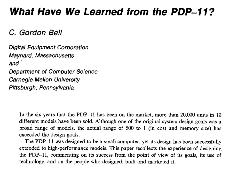
C. G. Bell, W. D. Strecker, “Computer What Have We Learned from the PDP-11,” The 3rd Annual Symposium on Computer Architecture Conference Proceedings, pp. l-14, 1976.
The paper I have chosen tonight is a retrospective on a computer design. It is one of a series of papers by Gordon Bell, and various co-authors, spanning the design, growth, and eventual replacement of the companies iconic line of PDP-11 mini computers.
- C. G. Bell, R. Cady, H. McFarland, B. Delagi, J. O’Laughlin, R. Noonan and W. Wulf, “A New Architecture for Mini-Computers – The DEC PDP- 11,” Proceedings of the Sprint Joint Computer Conference, pp. 657-675, AFIPS Press, 1970.
- C. G. Bell, W. D. Strecker, “Computer What Have We Learned from the PDP-11,” The 3rd Annual Symposium on Computer Architecture Conference Proceedings, pp. l-14, 1976.
- W. D. Strecker, “VAX-11/780: A Virtual Address Extension to the DEC PDP-11 Family,” Proceedings of the National Computer Conference, pp. 967-980, AFIPS Press, 1978.
- C. G. Bell, W. D. Strecker, “Retrospective: what have we learned from the PDP-11—what we have learned from VAX and Alpha”, Proceedings of the 25th Annual International Symposium on Computer Architecture, pp. 6-10, 1998.
This year represents the 60th anniversary of the founding of the company that produced the PDP-11. It is also 40 years since this paper was written, so I thought it would be entertaining to review Bell’s retrospective through the lens of our own 20/20 hindsight.
Image credit: saccade.com
Who were Digital Equipment Corporation?
To set the scene for this paper, first we should talk a little about the company that produced the PDP-11, the Digital Equipment Corporation of Maynard, Massachusetts. Better known as DEC.
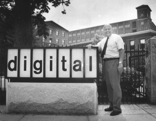
Image Credit: boston.com
DEC was founded in 1957 by Ken Olsen, and Harlan Anderson. Olsen and Anderson had worked together at MIT’s Lincoln Laboratory where they noticed that students would queue for hours to use the TX-0, an experimental interactive computer designed by Wes Clarke.
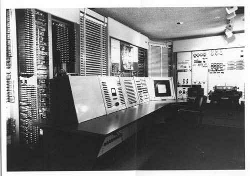
Image credit: computerhistory.org
This is the TX-0. What do you notice about it?
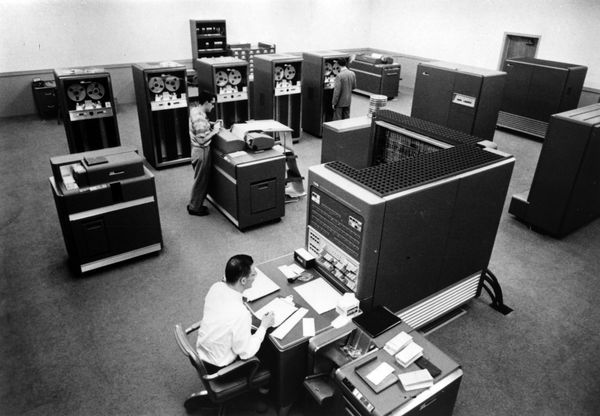
Image credit: computerhistory.org
Let’s compare it to something like the IBM 704, a contemporary mainframe, which the MIT students largely ignored. What Olsen and Anderson recognised was the desire for an interactive computer experience was so strong that there was a market for “small” computers dedicated to this role.
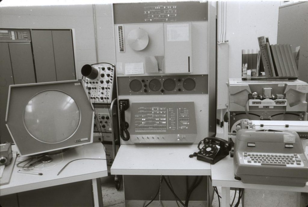
Image credit: computer-history.info
DEC’s first offering was the PDP-1, effectively a commercial version of the TX-0.
Correction: Michael Cheponis, the lead on the PDP-1 restoration project, kindly wrote to me with the following information.
Whirlwind and PDP-1 have 5 bit operation codes, TX-0 started with a 2 or 3 bit operation code, but gradually grew more after it lost the large memory to TX-2. A comparison of the PDP-1 and Whirlwind order codes makes it clear that the PDP-1 is a cost reduced and slightly improved version of the Whirlwind architecture.
-
- Improvement: add indirect addressing.
- Cost reduction: eliminate the live register by adding the subroutine call instructions, and eliminate the shift counter by replacing integer multiply and divide with multiply step and divide step instructions and making the shift instructions shift once for each bit in the address field.The biggest cost reduction was due to taking advantage of the advancement in logic design and packaging from Whirlwind to the PDP-1. (Using the Barta building for packaging versus 4 standard electronics racks.)
The contrast between the PDP-1 and the IBM 704 was visible at MIT, but the small, slow interactive computers, the Librascope LGP-30 and the Bendix G-15 preceded the PDP-1 by several years and sold in similar quantities.
It’s also worth noting that the name PDP is an acronym for “Programmed Data Processor”, as at the time, computers had a reputation of being large, complicated, and expensive machines, and DEC’s venture capitalists would not support them if they built a “computer”.
Following the success of the PDP-1, DEC’s offerings blossomed into several families of computers, many of which were designed at least in part by Gordon Bell, the author of tonight’s paper.
Introduction
A computer is not solely determined by its architecture; it reflects the technological, economic, and human aspects of the environment in which it was designed and built. […] The finished computer is a product of the total design environment.
Right from the get go, Bell is letting us know that the success of any computer project is not abstractly building the best computer but building the right computer, and that takes context.
In this chapter, we reflect on the PDP-11: its goals, its architecture, its various implementations, and the people who designed it. We examine the design, beginning with the architectural specifications, and observe how it was affected by technology, by the development organization, the sales, application, and manufacturing organizations, and the nature of the final users.
By this time, 1976, Bell has been the VP of engineering at DEC for nearly four years. It’s clear that he’s considering the success of the PDP-11 in the wider context of the market which it was both developed to serve, and which would later influence the evolution of the PDP-11 line.
In keeping with the spirit of Bell’s words, this presentation focuses on two aspects of the paper; the technology and the people.
Background: Thoughts Behind The Design
Bell opens with this observation
It is the nature of computer engineering to be goal-oriented, with pressure to produce deliverable products. It is therefore difficult to plan for an extensive lifetime.
This is your agile mindset, right here. This is 25 years before Snowbird and the birth of the Agile manifesto. When this was written DEC weren’t a scrappy startup desperate to make their bones, they were an established company with several successful product lines in the market, and Bell is talking about the pressure to ship a minimum viable product trampling all over notions of being able to plan elaborately.
Like the IBM/360, the PDP-11 was designed not just as a single model of computer, but a range of models, for which software written for a small PDP-11 would be compatible with the larger one.
“The term architecture is used here to describe the attributes of a system as seen by the programmer, i.e., the conceptual structure and functional behaviour, as distinct from the organisation of the data flow and controls, the logical design, and the physical implementation.” — G. M. Amdahl G. A. Blaauw and F. P. Brooks Jr. Architecture of the IBM System/360, 1964
Because of the open nature of the PDP-11, anything which interpreted the instructions according to the processor specification, was a PDP-11, so there had been a rush within DEC, once it was clear that the PDP-11 market was heating up, to build implementations; you had different groups building fast, expensive ones and cost reduced slower ones.
Despite its evolutionary planning, the PDP-11 has been quite successful in the marketplace: over 20,000 have been sold in the six years that it has been on the market (197Cb1975). It is not clear how rigorous a test (aside from the marketplace) we have given the design, since a large and aggressive marketing organization, armed with software to correct architectural inconsistencies and omissions, can save almost any design.
Here Bell is introducing his hypothesis for the paper; was the PDP-11 a great design, or was it simply the beneficiary of a hyperactive marketing department? To answer his own question Bell begins to reflect on the product that emerged and evaluate it against the design criteria that he and his fellow authors identified six years earlier.
Address space
The first weakness of minicomputers was their limited addressing capability. The biggest (and most common) mistake that can be made in a computer design is that of not providing enough address bits for memory addressing and management.
Minicomputers of the era often came with a 12 bit address space, offering just 4096 addresses each holding a 12 bit value called a word.
It’s worth taking an aside to note that the word minicomputer, which later came to be understood to be an indication of their physical size, was originally a contraction of the words minimal computer. The canonical example was the PDP-8, DEC’s previous offering, which offered just eight instructions.
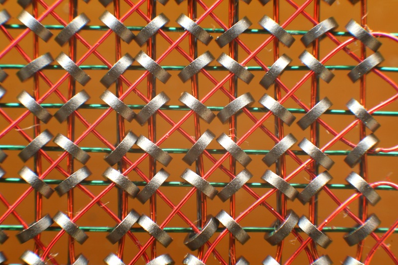
Image credit: wikipedia
The reason for this tiny address spaces was cost. Memory was extremely expensive in the 60’s and early 70’s as each bit of storage consisted of a tiny iron doughnut, or core, woven into a mesh of control wires.
Cores were arranged into a plane, in this case representing 4096 bits, then stacked to produce words, so a 4096 word memory contained 16 million cores, all of which were at least partially hand assembled. You can see why memory was expensive.
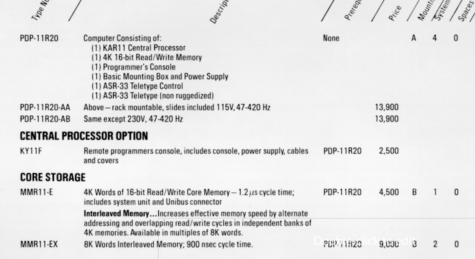
Image credit: bitsavers.org
Bell and the other PDP-11 designers knew that core memory prices were continuing to fall, and that semiconductor memory, while not cost effective at that time, would continue to drive down the price per bit of storage. Thus the amount of memory that customers could afford to buy would increase over time as “… users tend to buy “constant dollar” systems”. But alas,
The PDP-11 followed this hallowed tradition of skimping on address bits, but it was saved by the principle that a good design can evolve through at least one major change.
Even with the designers foresight, Bell noted that not two years after its introduction, the PDP-11 had to be redesigned to include a memory management unit to allow access to a larger 18 bit address space at the cost of increased programming complexity. A few years later a further 4 bits were added.
In fairness, while Bell chastised himself for not seeing this coming, this pattern of insufficient address bits continues to this day. Who remembers the dos 640k limit? Who remembers fighting with himem.sys? Who has struggled with 32 bit programs that need more than 2gb of heap?
So, none of us are perfect.
Insufficient registers
A second weakness of minicomputers was their tendency not to have enough registers. This was corrected for the PDP-11 by providing eight 16-bit registers. Later, six 32-bit registers were added for floating-point arithmetic. […] More registers would increase the multiprogramming context switch time and confuse the user.
It was not uncommon, even for mainframes of the day, to offer only a single register—the accumulator. If additional registers were provided, they would be specifically for use in indexing operations, they were not general purpose.
It’s also interesting to note Bell’s concern that additional registers would confuse the user. In the early 1970’s the assumption that the machine would be programmed directly in assembly was still the prevailing mindset.
There is a strong interplay between the number of registers in an architecture, the number of address bits, and the size of the instruction. All of these factors are rooted in the scarcity of memory, so it’s worth taking a little detour into instruction set design.
In Von Neumann machines (of which almost all computers of the 60’s were) the program and its data share the same, limited, address space, so inefficient programs didn’t just waste computing time, they wasted memory. A slow program is somewhat tolerable, but a program that is too large to fit in memory is a fatal condition, so you want your instruction encoding to be as efficient as possible.
Let’s consider the very common case of moving an value from one location in memory to another. How many bits would you need to describe that operation? One implementation might be:
MOV <addr> <addr>
Which would take 16 bits for the source, and a further 16 for the destination, and the some bits to encode the MOV instruction itself. Let’s call it 40 bits; this is not a multiple of 16, which would mean a complicated 2.5 word instruction encoding. However, what if we were to load that address into a register?
MOV (R0), (R1)
Then we’d only need to describe the register, the PDP had 8 registers, so only 3 bits per register, plus some for the operator. This could easily fit into a 16 bit word, rather than requiring a complex variable length encoding.
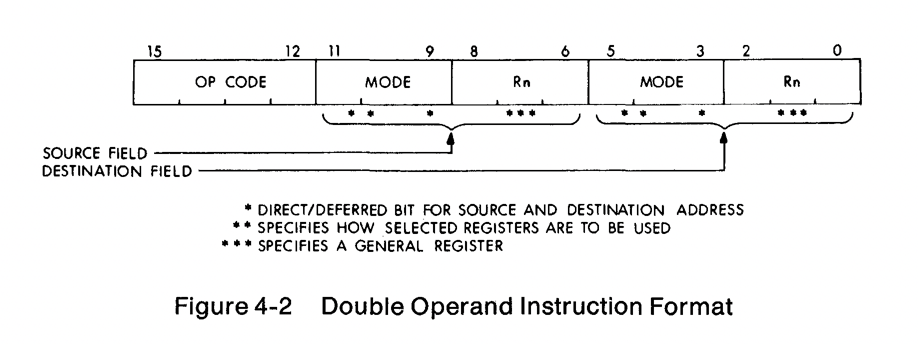
Image credit: bitsavers.org
It actually turns out that the PDP-11 uses 6 bits per register, but that still left 4 bits for the operation when two operands were present.
Hardware stack
A third weakness of minicomputers was their lack of hardware stack capability. In the PDP-11, this was solved with the autoincrement/autodecrement addressing mechanism. This solution is unique to the PDP-11 and has proven to be exceptionally useful. (In fact, it has been copied by other designers.)
Nowadays it’s hard to imagine hardware that doesn’t have a notion of a stack, but consider that a stack isn’t important if you don’t need recursion.
The design for the PDP-11 was laid down in 1969 and if we look at the programming languages of the time, FORTRAN and COBOL, neither supported recursive function calls. The function call sequence would often store the return address at a blank word at the start of the procedure making recursion impossible.
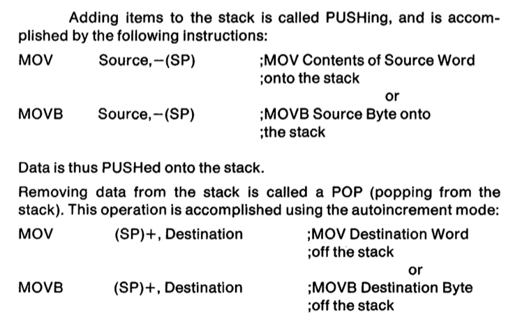
Image credit: bitsavers.org
The PDP-11 defined a stack pointer as we understand today, a register that controlled the operation of PUSH and POP style instructions, but the PDP-11 went one better and permitted any register to operate as a stack pointer by the addition of an auto increment/decrement modifier on all register operands.
For example, this single instruction:
MOV R4, -(R6)
will decrement the value stored in R6 by two, then store the value in R4 into the address stored in R6. This is the how you push a value onto the stack in PDP-11 assembler. If anyone has done any ARM programming, this will be very familiar to you.
This means there is no need for a dedicated PUSH or POP instruction, saving instruction encoding space, and allowing any register to be used as a stack pointer, although traditionally R6 was assumed by the hardware if you used the native subroutine call instruction.
Interrupt latency
A fourth weakness, limited interrupt capability and slow context switching, was essentially solved with the device of UNIBUS interrupt vectors, which direct device interrupts.
At this point in DEC’s lifetime, almost all of its products, save the PDP-10 which was DEC’s mainframe offering, were aimed at interactive, laboratory, or process control applications. Interrupt responsiveness, the delay between an interrupt signal being raised, and the computer being ready to process the interrupt, is key to real time performance.
The PDP-11 addressed this by permitting the device that raised the interrupt to supply the address to service the interrupt. Bell proudly reported that:
The basic mechanism is very fast, requiring only four memory cycles from the time an interrupt request is issued until the first instruction of the interrupt routine begins execution.
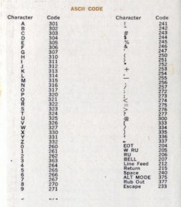
Character handling
A fifth weakness of prior minicomputers, inadequate character-handling capability, was met in the PDP-11 by providing direct byte addressing capability.
Strings and character handling were of increasing importance during the 1960’s as scientific and business computing converged. The predominant character encodings at the time were 6 bit character sets which provided just enough space for upper case letters, the digits 0 to 9, space, and a few punctuation characters sufficient for printing financial reports.
DEC Sixbit encoding
Because memory was so expensive, placing one 6 bit character into a 12 or 18 bit word was simply unacceptable so characters would be packed into words.
This proved efficient for storage, but complex for operations like move, compare, and concatenate, which had to account for a character appearing in the top or bottom of the word, expending valuable words of program storage to cope.
The problem was addressed in the PDP-11 by allowing the machine to operate on memory as both a 16-bit word, and the increasingly popular 8-bit byte. The expenditure of 2 additional bits per character was felt to be worth it for simpler string handling, and also eased the adoption of the increasingly popular 7-bit ASCII standard of which DEC were a proponent at the time. Bell concludes this point with the throw away line:
Although string instructions are not yet provided in the hard- ware, the common string operations (move, compare, concatenate) can be programmed with very short loops.
And indeed they can. One can write a string copy routine using two instructions, assuming that the source and destination are already in registers.
loop:   MOVB (src)+, (dst)+
        BNE loop
The routine takes full advantage of the fact that MOV updates the processor flag. The loop will continue until the value at the source address is zero, at which point the branch will fall through to the next instruction. This is why C strings are terminated with zeros.
Read only memory
A sixth weakness, the inability to use read-only memories, was avoided in the PDP-11. Most code written for the PDP-11 tends to be pure and reentrant without special effort by the programmer, allowing a read-only memory (ROM) to be used directly.
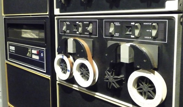
In process control applications, where the program is relatively fixed, having to load the program each time from magnetic or punched tape is expensive. You have to buy and maintain infrequently used I/O devices. It would be far more convenient if the program could always be present in the computer at startup. However, because of the extreme memory shortage of early minicomputers, and the lack of notion of a hardware stack, self modifying code was often unavoidable, which seriously limited the use of read only memory. Bell is justifiably proud that the PDP-11 design knocked that one out of the park.
Primitive I/O Capabilities
A seventh weakness, one common to many minicomputers, was primitive I/O capabilities.
During the late 60’s when the PDP-11 was being designed, input/output was very expensive. Mainframes of the time use a model called channel I/O, where the main CPU sent a small program to a channel controller, which would execute the program and report the result. The program would usually instruct a tape drive to load a record, or a punch to punch a card.
Channel I/O was important because it allowed the mainframe to offload the oversight of the I/O operation to another processor, freeing its valuable cycles, and permitting overlapping I/O, which in turn increased processor utilisation. The downside was channel I/O required a smaller CPU inside each channel controller which increased the cost of the installation substantially.
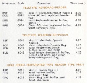 In the minicomputer world, I/O was usually performed directly by the CPU, usually with specialised instructions hard coded for a specific device, eg. the paper tape reader or console printer.
The PDP-11 introduced something unique, memory mapped I/O. This isn’t memory mapped I/O that you might be used to with the mmap(2) system call, but rather the convention that specific addresses in memory weren’t just dumb storage, instead their contents were mapped onto cards plugged into the backplane, which DEC called the UNIBUS.
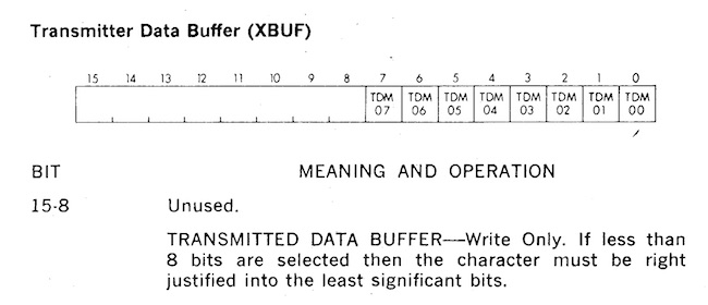
Image credit: bitsavers.org
For example, a value written to 777566 would be written to device attached to the console, usually a hard copy terminal.
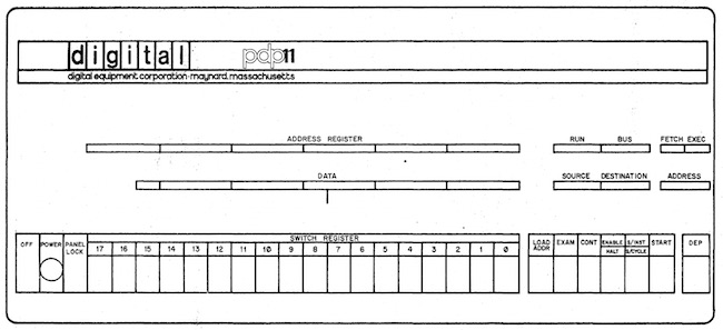
Image credit: bitsavers.org
If you read the value at address 777570, you get the value entered on the front panel switches. This was often used as an early form of bootstrap configuration.
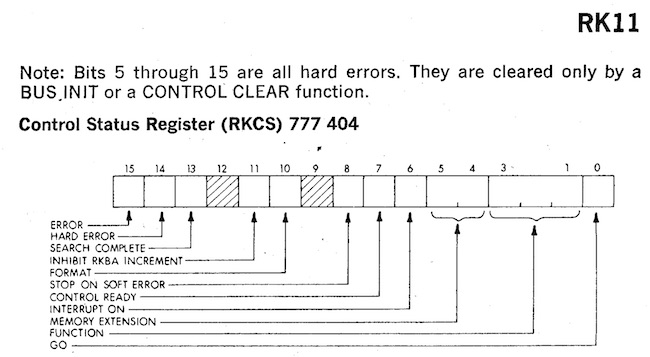
Image credit: bitsavers.org
Similarly talking to the RK05 disk drive was accomplished by writing the sector number you wanted to access to 777412, the address to transfer that sector to address 777410, and the number of words to 777406. Then by setting bit zero at address 777404 to 1 (the GO bit), the drive will transfer the number of words you asked for directly into memory.
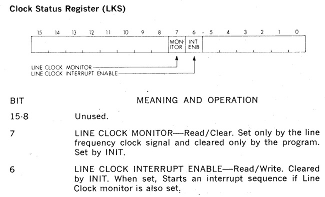
Image credit: bitsavers.org
My favorite has got to be the KW11-L line clock. A write to bit 6 of address 777546 starts an interrupt firing every 20ms. What’s special about 20ms? Because that’s the reciprocal of the frequency of the AC waveform here in the US. Yup, just like a bedside clock, the PDP-11 told time by counting the number of power line cycles.
High programming costs
A ninth weakness of minicomputers was the high cost of programming them. Many users program in assembly language, without the comfortable environment of editors, file systems, and debuggers available on bigger systems. The PDP-11 does not seem to have overcome this weakness, although it appears that more complex systems are being built successfully with the PDP-11 than with its predecessors, the PDP-8 and PDP-15.
Because of their minimal nature, mini computers were not pleasant environments on which to write programs. Often this would involve tedious switch flipping, or perhaps editing and assembling a program on another, larger, computer and then transferring it via paper tape.
This is very much akin to how those of us who work with micro controllers are still programming today; editing on a large workstation, compiling a target hex file, then transferring that hex to the micro controller’s flash storage.
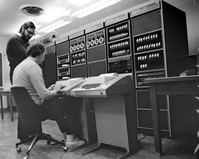
Image credit: Dennis Ritchie
However, it seems Bell was unaware of the work of Thompson and Ritchie, who were busy constructing their own programming environment on their PDP-11 in New Jersey.
People: Builders of the Design
Now we move to the second section; the people.
As an amateur historian this section is the most interesting to me, because the study of the history of computing, or really any historical subject, is fundamentally a study of people, and the context surrounding the decisions they made.
Bell recognises that while computers are built from technology, they are built by people and thus he dedicates this section to describing the group dynamics at DEC during the development of the PDP-11.
The problems faced by computer designers can usually be attributed to one of two causes: inexperience or second-systemitis.
Here Bell recalls the words of Fred Brooks from his recent (at the time) book The Mythical Man-Month.
Brooks, the lead for the OS/360 project struggled for years to build a single general purpose operating system that would run across the entire range of IBM/360 modes, this was after all the goal of the 360 project. Brooks’ words must have been fresh in Bell’s mind when he wrote this paragraph.
Chronology of the design
This section is a perfect window into the operation of DEC in the late 1960’s
The internal organization of DEC design groups has through the years oscillated between market orientation and product orientation. Since the company has been growing at a rate of 30 to 40% a year, there has been a constant need for reorganization. At any given time, one third of the staff has been with the company less than a year.
Raise your hand if this sounds familiar to you.
At the time of the PDP-11 design, the company was structured along product lines. The design talent in the company was organized into tight groups: the PDP-10 group, the PDP-15 (an 18-bit machine) group, the PDP-8 group, an ad hoc PDP-8/S subgroup, and the LINC-8 group. Each group included marketing and engineering people responsible for designing a product, software and hardware. As a result of this organization, architectural experience was diffused among the groups, and there was little understanding of the notion of a range of products.
Here Bell spends some time iterating through each group, listing their strengths and weaknesses as sponsors for the PDP-11. I won’t recount all the choices, with one exception.
The PDP-10 group was the strongest group in the company. They built large powerful time-shared machines. It was essentially a separate division of the company, with little or no interaction with the other groups. Although the PDP-10 group as a whole had the best understanding of system architectural controls, they had no notion of system range, and were only interested in building higher-performance computers.
Having recently worked for a software company where one or two of the oldest products made almost all the company profit I have some sympathy for Bell’s position. The PDP-10 was DEC’s version of a mainframe; enormously powerful, but was only available at one price point.
The first design work for a 16-bit computer was carried out under the eye of the PDP-15 manager, a marketing person with engineering background. This first design was called PDP-X, and included specification for a range of machines. As a range architecture, it was better designed than the later PDP-11, but was not otherwise particularly innovative. Unfortunately, this group managed to convince management that their design was potentially as complex as the PDP-10 (which it was not), and thus ensured its demise, since no one wanted another large computer unrelated to the company’s main large computer.
And here Bell teaches us an important lesson; when your competition is in the same reporting chain, they have effective tools to ensure your project is killed before it reaches the market.
In retrospect, the people involved in designing PDP-X were apparently working simultaneously on the design of Data General.
This shade might go unnoticed by the casual reader, but it’s a reference to a defection to rival that of Shockely’s traitorous eight a decade earlier.
Edson de Castro, the product manager of the PDP-8, and lead on the PDP-X project had left DEC, along with several of his team to form Data General. The record is not clear if de Castro left because the PDP-X was canceled or if his departure was the final straw for the faltering project. In either case, the result was obvious, as Bell writes.
As the PDP-X project folded, the DCM (Desk Calculator Machine, a code name chosen for security) was started. Design and planning were in disarray, as Data General had been formed and was competing with the PDP-8, using a very small 16-bit computer.
Data General were now competing with DEC with their 16 bit Nova in the space that the PDP-8 had defined and de Castro knew like the back of his hand; rack mounted laboratory equipment.
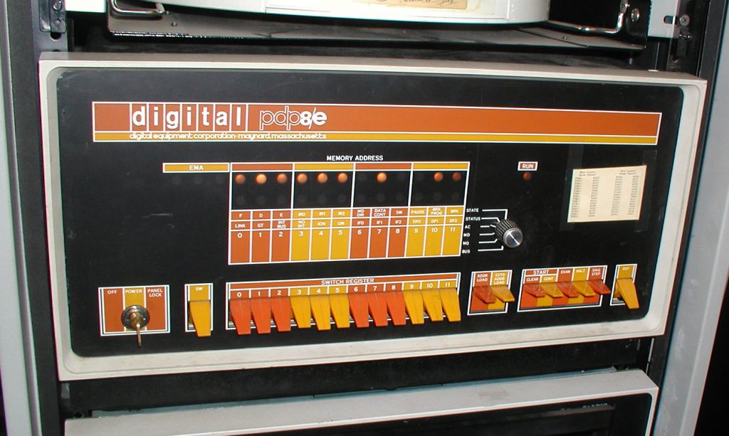
Image credit: vintagecomputer.net
The 12 bit PDP-8 versus Data General’s 16 bit Nova
The PDP-11: An Evaluation
The last section of the paper, having evaluated the PDP-11 against its predecessors, Bell proceeds to evaluate the PDP-11 against itself. The biggest take away was the UNIBUS.
In general, the UNIBUS has behaved beyond all expectations. Several hundred types of memories and peripherals have been interfaced to it; it has become a standard architectural component of systems in the $3K to $100K price range (1975).
What is the UNIBUS?
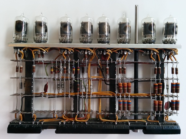
Image credit: wikipedia
The earliest commercial computers were designed with plugin modules connected by a wired backplane. In the days of vacuum tubes this was a necessity because of the unreliability of tubes and the need to replace modules quickly.
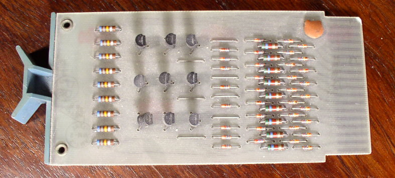
Image credit: wikipedia
Later a desire to build computers out of a standardized modules resulted in the generalised logic blocks interconnected by a sophisticated backplane. This is an example of DEC’s early flip-chip offerings.
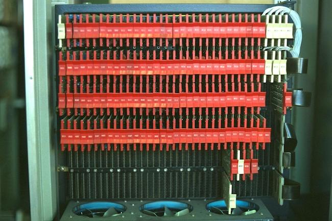
Image credit: piercefuller.com
You’d mount them on a complex wire wrapped backplane to build a computer, in this case a PDP-8.
The UNIBUS represented an evolution of the previous DEC designs as an abstraction of an idealised control plane. The availability of medium scale integrated components moved the complexity from the backplane to the modules that populated it. This in turn created a standard way for additional modules to be attached to the computer.
The UNIBUS, as a standard, has provided an architectural component for easily configuring systems. Any company, not just DEC, can easily build components that interface to the bus. Good buses make good engineering neighbours, since people can concentrate on structured design. Indeed, the UNIBUS has created a secondary industry providing alternative sources of supply for memories and peripherals. With the exception of the IBM 360 Multiplexor/Selector bus, the UNIBUS is the most widely used computer interconnection standard.
Prior to the UNIBUS, the I/O devices a minicomputer could support were dictated by the designers. You almost had to encode how to talk to them into the CPU logic. After the UNIBUS, the field for end user customisation and experimentation was cracked wide open.
What have we learned from the PDP-11?
Bell’s retrospective ended when the paper was written in 1976/77, but from our vantage point, forty years later, the impact that the PDP-11 has been huge.
RISC
First of all, while the PDP-11 was not designed, or even understood to be a RISC processor–that term would not be coined util 1976 by John Cocke and the IBM 801. However to anyone with experience with processors like the ARM, a contemporary RISC microprocessor, the similarities between the two instruction sets are striking. Just as programming language design is a process of evolution and cultural poaching, so too it seems is instruction set design.
The PDP-11 also drove a stake firmly through the heart of dedicated I/O instructions, it cemented the model of memory mapped I/O as the predominant control mechanism to this day. The only processors post the PDP that offered seperate input/output instructions that I can think of were the Intel 8080, and its cousin, the Z80.
UNIX
Next is the PDP-11’s impact on software and operating systems. The PDP-11 is the machine on which Ken Thompson and Dennis Ritchie developed UNIX at Bell Labs.
Before the PDP-11, there was no UNIX. Before the PDP-11, there was no C, this is the computer that C was designed on. If you want to know why the classical C int is 16 bits wide, it’s because of the PDP-11.
UNIX bought us ideas such as pipes, everything is a file, and interactive computing.
VAX-11/780
In interactive computing, memory usage is effectively unbounded, and while the PDP was perfect for process control applications, this demand for interactive computing was the hallmark and driver for the PDP-11’s replacement.
The year this paper was released, 1977, the PDP-11’s successor, the VAX-11, which stood for “virtual address extension”–you can see Bell was not going to address space mistake again–was released.
BSD
UNIX, which had arrived at Berkley in 1974 aboard a tape carried by Ken Thompson, would evolve into the west coast flavoured Berkley Systems Distribution.
Berkeley UNIX had been ported to the VAX by the start of the 1980’s and was thriving as the counter cultural alternative to DEC’s own VMS operating system. Berkeley UNIX spawned a new generation of hackers who would go on to form companies like Sun micro systems, and languages like Self, which lead directly to the development of Java.
UNIX was ported to a bewildering array of computer systems during the 80’s and the fallout from the UNIX wars gave us the various BSD operating systems who continue to this day.
NeXT
4BSD, a descendant of the original Berkeley distribution became the basis of the operating system for Steve Job’s NeXT line of computers. And when Apple purchased NeXT in 1997, NextSTEP and its BSD derived user space, became the foundations for Darwin, OSX, and iOS.
Windows NT
As we say earlier with Edson de Castro, DEC was no stranger to breakups.
Dave Cutler, the architect of the VAX VMS operating system, after a failed attempt to start a new combined operating system and hardware project, designed to succeed the VAX, decamped to Microsoft in 1988 bringing with him his team and lead the development of Windows NT. Those with a knowledge of Windows’ internals and VMS will perhaps spot the similarities.
Xerox Alto
To close the loop on the de Castro story, the Data General Nova series provided inspiration to Charles Thacker and Butler Lampson, the designers of the Xerox Alto, which itself was the fabled inspiration for the look and feel of the Apple Macintosh.
Data General Nova
The rivalry between Data General and DEC continued into the 32 bit era, the story of which is told in Tracy Kidder’s 1981 Pulitzer winner, The Soul of a New Machine.
What have we learned from the PDP-11?
While its development was sometimes chaotic, and not without its flaws, the PDP-11 is at the intersection of many threads of history.
Hardware, software, programming languages, operating systems, have all been influenced by the PDP-11. I wager there is not a single person in this room who cannot trace the lineage of the language they work with, the computer they use, or the operating system it runs, back to the PDP-11.
And that is worth celebrating.
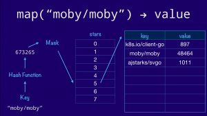
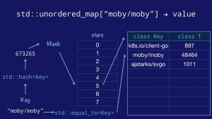
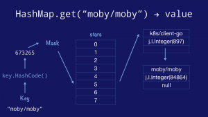
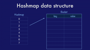 The classical hashmap is an array of buckets each of which contains a pointer to an array of key/value entries. In this case our hashmap has eight buckets (as this is the value that the Go implementation uses) and each bucket can hold up to eight entries each (again drawn from the Go implementation). Using powers of two allows the use of cheap bit masks and shifts rather than expensive division.
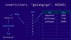
