Overview
The goal for this workshop is to give you the tools you need to diagnose performance problems in your Go applications and fix them.
Through the day we’ll work from the small — learning how to write benchmarks, then profiling a small piece of code. Then step out and talk about the execution tracer, the garbage collector and tracing running applications. The remainder of the day will be a chance for you to ask questions, experiment with your own code.
|
You can find the latest version of this presentation at |
Schedule
Here’s the (approximate) schedule for the day.
| Start | Description |
|---|---|
09:00 |
Welcome and Introduction |
09:30 |
|
10:45 |
Break (15 minutes) |
11:00 |
|
12:00 |
Lunch (90 minutes) |
13:30 |
|
14:30 |
|
15:30 |
Break (15 minutes) |
15:45 |
|
16:15 |
|
16:30 |
Exercises |
16:45 |
|
17:00 |
Close |
Welcome
Hello and welcome! 🎉
The goal for this workshop is to give you the tools you need to diagnose performance problems in your Go applications and fix them.
Through the day we’ll work from the small — learning how to write benchmarks, then profiling a small piece of code. Then step out and talk about the execution tracer, the garbage collector and tracing running applications. The remainder of the day will be a chance for you to ask questions, experiment with your own code.
Instructors
-
Dave Cheney dave@cheney.net
License and Materials
This workshop is a collaboration between David Cheney and Francesc Campoy.
This presentation is licensed under the Creative Commons Attribution-ShareAlike 4.0 International licence.
Prerequisites
The are several software downloads you will need today.
The workshop repository
Download the source to this document and code samples at https://github.com/davecheney/high-performance-go-workshop
Laptop, power supplies, etc.
The workshop material targets Go 1.12.
| If you’ve already upgraded to Go 1.13 that’s ok. There are always some small changes to optimisation choices between minor Go releases and I’ll try to point those out as we go along. |
Graphviz
The section on pprof requires the dot program which ships with the graphviz suite of tools.
-
Linux:
[sudo] apt-get install graphviz -
OSX:
-
MacPorts:
sudo port install graphviz -
Homebrew:
brew install graphviz -
Windows (untested)
Google Chrome
The section on the execution tracer requires Google Chrome. It will not work with Safari, Edge, Firefox, or IE 4.01. Please tell your battery I’m sorry.
Your own code to profile and optimise
The final section of the day will be an open session where you can experiment with the tools you’ve learnt.
One more thing …
This isn’t a lecture, it’s a conversation. We’ll have lots of breaks to ask questions.
If you don’t understand something, or think what you’re hearing not correct, please ask.
1. The past, present, and future of Microprocessor performance
This is a workshop about writing high performance code. In other workshops I talk about decoupled design and maintainability, but we’re here today to talk about performance.
I want to start today with a short lecture on how I think about the history of the evolution of computers and why I think writing high performance software is important .
The reality is that software runs on hardware, so to talk about writing high performance code, first we need to talk about the hardware that runs our code.
1.1. Mechanical Sympathy

There is a term in popular use at the moment, you’ll hear people like Martin Thompson or Bill Kennedy talk about “mechanical sympathy”.
The name "Mechanical Sympathy" comes from the great racing car driver Jackie Stewart, who was a 3 times world Formula 1 champion. He believed that the best drivers had enough understanding of how a machine worked so they could work in harmony with it.
To be a great race car driver, you don’t need to be a great mechanic, but you need to have more than a cursory understanding of how a motor car works.
I believe the same is true for us as software engineers. I don’t think any of us in this room will be a professional CPU designer, but that doesn’t mean we can ignore the problems that CPU designers face.
1.2. Six orders of magnitude
There’s a common internet meme that goes something like this;

Of course this is preposterous, but it underscores just how much has changed in the computing industry.
As software authors all of us in this room have benefited from Moore’s Law, the doubling of the number of available transistors on a chip every 18 months, for 40 years. No other industry has experienced a six order of magnitude [1] improvement in their tools in the space of a lifetime.
But this is all changing.
1.3. Are computers still getting faster?
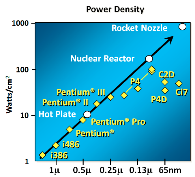
So the fundamental question is, confronted with statistic like the ones in the image above, should we ask the question are computers still getting faster?
If computers are still getting faster then maybe we don’t need to care about the performance of our code, we just wait a bit and the hardware manufacturers will solve our performance problems for us.
1.3.1. Let’s look at the data
This is the classic data you’ll find in textbooks like Computer Architecture, A Quantitative Approach by John L. Hennessy and David A. Patterson. This graph was taken from the 5th edition
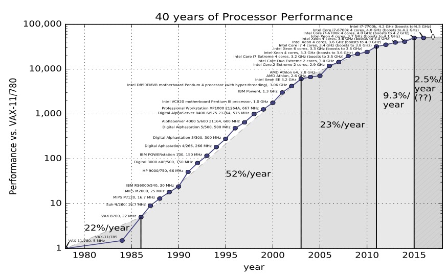
In the 5th edition, Hennessey and Patterson argue that there are three eras of computing performance
-
The first was the 1970’s and early 80’s which was the formative years. Microprocessors as we know them today didn’t really exist, computers were built from discrete transistors or small scale integrated circuits. Cost, size, and the limitations in the understanding of material science were the limiting factor.
-
From the mid 80s to 2004 the trend line is clear. Computer integer performance improved on average by 52% each year. Computer power doubled every two years, hence people conflated Moore’s law — the doubling of the number of transistors on a die, with computer performance.
-
Then we come to the third era of computer performance. Things slow down. The aggregate rate of change is 22% per year.
That previous graph only went up to 2012, but fortunately in 2012 Jeff Preshing wrote a tool to scrape the Spec website and build your own graph.
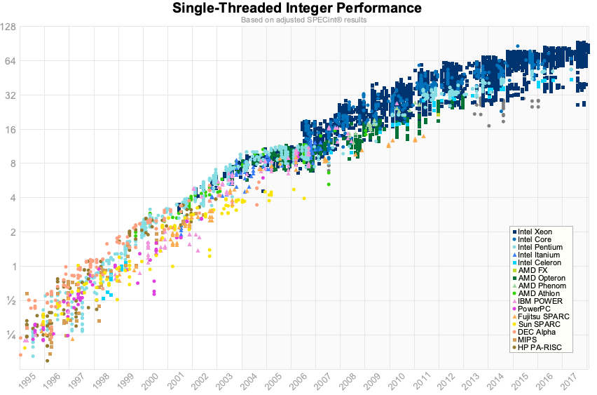
So this is the same graph using Spec data from 1995 til 2017.
To me, rather than the step change we saw in the 2012 data, I’d say that single core performance is approaching a limit. The numbers are slightly better for floating point, but for us in the room doing line of business applications, this is probably not that relevant.
1.3.2. Yes, computer are still getting faster, slowly
The first thing to remember about the ending of Moore’s law is something Gordon Moore told me. He said "All exponentials come to an end". — John Hennessy
This is Hennessy’s quote from Google Next 18 and his Turing Award lecture. His contention is yes, CPU performance is still improving. However, single threaded integer performance is still improving around 2-3% per year. At this rate its going to take 20 years of compounding growth to double integer performance. Compare that to the go-go days of the 90’s where performance was doubling every two years.
Why is this happening?
1.4. Clock speeds
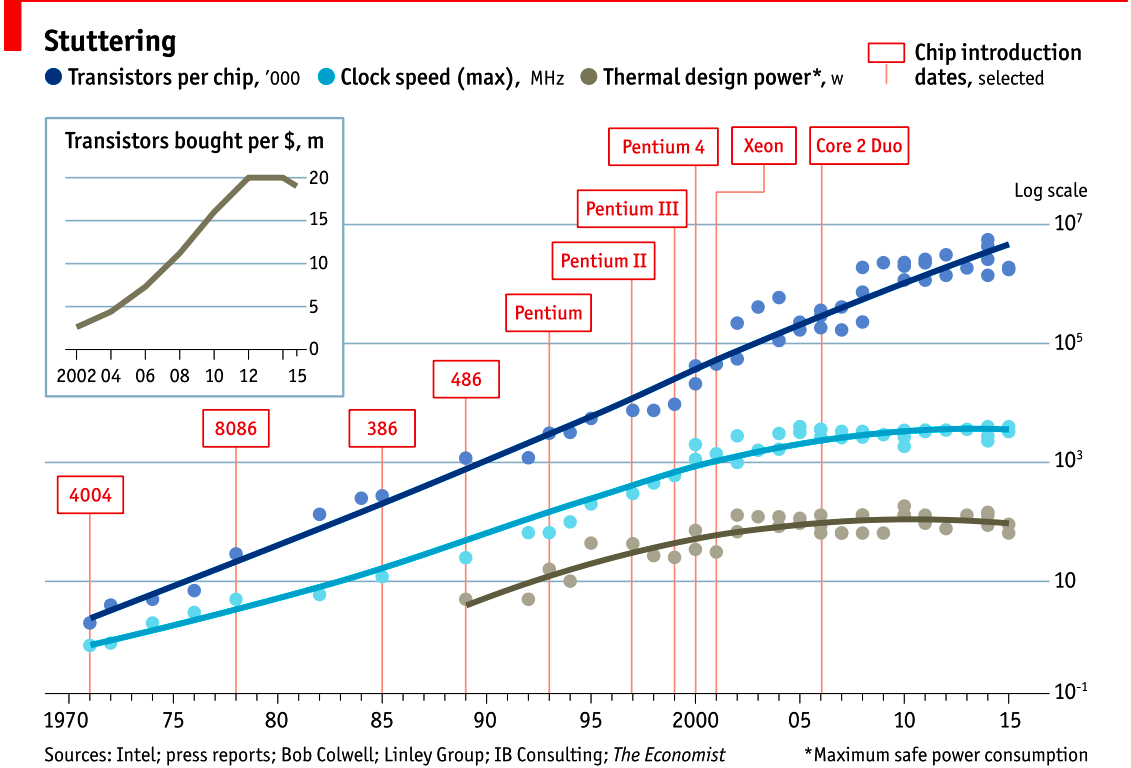
This graph from 2015 demonstrates this well. The top line shows the number of transistors on a die. This has continued in a roughly linear trend line since the 1970’s. As this is a log/lin graph this linear series represents exponential growth.
However, If we look at the middle line, we see clock speeds have not increased in a decade, we see that cpu speeds stalled around 2004
The bottom graph shows thermal dissipation power; that is electrical power that is turned into heat, follows a same pattern—clock speeds and cpu heat dissipation are correlated.
1.5. Heat
Why does a CPU produce heat? It’s a solid state device, there are no moving components, so effects like friction are not (directly) relevant here.
This digram is taken from a great data sheet produced by TI. In this model the switch in N typed devices is attracted to a positive voltage P type devices are repelled from a positive voltage.
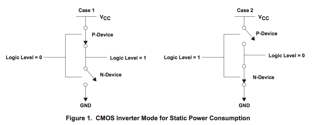
The power consumption of a CMOS device, which is what every transistor in this room, on your desk, and in your pocket, is made from, is combination of three factors.
-
Static power. When a transistor is static, that is, not changing its state, there is a small amount of current that leaks through the transistor to ground. The smaller the transistor, the more leakage. Leakage increases with temperature. Even a minute amount of leakage adds up when you have billions of transistors!
-
Dynamic power. When a transistor transitions from one state to another, it must charge or discharge the various capacitances it is connected to the gate. Dynamic power per transistor is the voltage squared times the capacitance and the frequency of change. Lowering the voltage can reduce the power consumed by a transistor, but lower voltages causes the transistor to switch slower.
-
Crowbar, or short circuit current. We like to think of transistors as digital devices occupying one state or another, off or on, atomically. In reality a transistor is an analog device. As a switch a transistor starts out mostly off, and transitions, or switches, to a state of being mostly on. This transition or switching time is very fast, in modern processors it is in the order of pico seconds, but that still represents a period of time when there is a low resistance path from Vcc to ground. The faster the transistor switches, its frequency, the more heat is dissipated.
1.6. The end of Dennard scaling
To understand what happened next we need to look to a paper written in 1974 co-authored by Robert H. Dennard. Dennard’s Scaling law states roughly that as transistors get smaller their power density stays constant. Smaller transistors can run at lower voltages, have lower gate capacitance, and switch faster, which helps reduce the amount of dynamic power.
So how did that work out?
It turns out not so great. As the gate length of the transistor approaches the width of a few silicon atom, the relationship between transistor size, voltage, and importantly leakage broke down.
It was postulated at the Micro-32 conference in 1999 that if we followed the trend line of increasing clock speed and shrinking transistor dimensions then within a processor generation the transistor junction would approach the temperature of the core of a nuclear reactor. Obviously this is was lunacy. The Pentium 4 marked the end of the line for single core, high frequency, consumer CPUs.
Returning to this graph, we see that the reason clock speeds have stalled is because cpu’s exceeded our ability to cool them. By 2006 reducing the size of the transistor no longer improved its power efficiency.
We now know that CPU feature size reductions are primarily aimed at reducing power consumption. Reducing power consumption doesn’t just mean “green”, like recycle, save the planet. The primary goal is to keep power consumption, and thus heat dissipation, below levels that will damage the CPU.
But, there is one part of the graph that is continuing to increase, the number of transistors on a die. The march of cpu features size, more transistors in the same given area, has both positive and negative effects.
Also, as you can see in the insert, the cost per transistor continued to fall until around 5 years ago, and then the cost per transistor started to go back up again.

Not only is it getting more expensive to create smaller transistors, it’s getting harder. This report from 2016 shows the prediction of what the chip makers believed would occur in 2013; two years later they had missed all their predictions, and while I don’t have an updated version of this report, there are no signs that they are going to be able to reverse this trend.
It is costing intel, TSMC, AMD, and Samsung billions of dollars because they have to build new fabs, buy all new process tooling. So while the number of transistors per die continues to increase, their unit cost has started to increase.
|
Even the term gate length, measured in nano meters, has become ambiguous. Various manufacturers measure the size of their transistors in different ways allowing them to demonstrate a smaller number than their competitors without perhaps delivering. This is the Non-GAAP Earning reporting model of CPU manufacturers. |
1.7. More cores
With thermal and frequency limits reached it’s no longer possible to make a single core run twice as fast. But, if you add another cores you can provide twice the processing capacity — if the software can support it.
In truth, the core count of a CPU is dominated by heat dissipation. The end of Dennard scaling means that the clock speed of a CPU is some arbitrary number between 1 and 4 Ghz depending on how hot it is. We’ll see this shortly when we talk about benchmarking.
1.8. Amdahl’s law
CPUs are not getting faster, but they are getting wider with hyper threading and multiple cores. Dual core on mobile parts, quad core on desktop parts, dozens of cores on server parts. Will this be the future of computer performance? Unfortunately not.
Amdahl’s law, named after the Gene Amdahl the designer of the IBM/360, is a formula which gives the theoretical speedup in latency of the execution of a task at fixed workload that can be expected of a system whose resources are improved.

Amdahl’s law tells us that the maximum speedup of a program is limited by the sequential parts of the program. If you write a program with 95% of its execution able to be run in parallel, even with thousands of processors the maximum speedup in the programs execution is limited to 20x.
Think about the programs that you work on every day, how much of their execution is parralisable?
1.9. Dynamic Optimisations
With clock speeds stalled and limited returns from throwing extra cores at the problem, where are the speedups coming from? They are coming from architectural improvements in the chips themselves. These are the big five to seven year projects with names like Nehalem, Sandy Bridge, and Skylake.
Much of the improvement in performance in the last two decades has come from architectural improvements:
1.9.1. Out of order execution
Out of Order, also known as super scalar, execution is a way of extracting so called Instruction level parallelism from the code the CPU is executing. Modern CPUs effectively do SSA at the hardware level to identify data dependencies between operations, and where possible run independent instructions in parallel.
However there is a limit to the amount of parallelism inherent in any piece of code. It’s also tremendously power hungry. Most modern CPUs have settled on six execution units per core as there is an n squared cost of connecting each execution unit to all others at each stage of the pipeline.
1.9.2. Speculative execution
Save the smallest micro controllers, all CPUs utilise an instruction pipeline to overlap parts of in the instruction fetch/decode/execute/commit cycle.
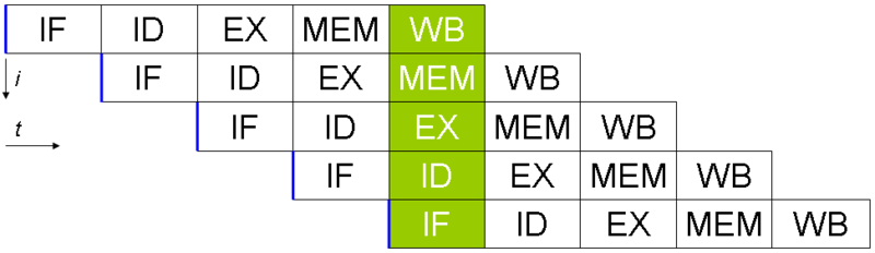
The problem with an instruction pipeline is branch instructions, which occur every 5-8 instructions on average. When a CPU reaches a branch it cannot look beyond the branch for additional instructions to execute and it cannot start filling its pipeline until it knows where the program counter will branch too. Speculative execution allows the CPU to "guess" which path the branch will take while the branch instruction is still being processed!
If the CPU predicts the branch correctly then it can keep its pipeline of instructions full. If the CPU fails to predict the correct branch then when it realises the mistake it must roll back any change that were made to its architectural state. As we’re all learning through Spectre style vulnerabilities, sometimes this rollback isn’t as seamless as hoped.
Speculative execution can be very power hungry when branch prediction rates are low. If the branch is misprediction, not only must the CPU backtrace to the point of the misprediction, but the energy expended on the incorrect branch is wasted.
All these optimisations lead to the improvements in single threaded performance we’ve seen, at the cost of huge numbers of transistors and power.
| Cliff Click has a wonderful presentation that argues out of order and speculative execution is most useful for starting cache misses early thereby reducing observed cache latency. |
1.10. Modern CPUs are optimised for bulk operations
Modern processors are a like nitro fuelled funny cars, they excel at the quarter mile. Unfortunately modern programming languages are like Monte Carlo, they are full of twists and turns. — David Ungar
This a quote from David Ungar, an influential computer scientist and the developer of the SELF programming language that was referenced in a very old presentation I found online.
Thus, modern CPUs are optimised for bulk transfers and bulk operations. At every level, the setup cost of an operation encourages you to work in bulk. Some examples include
-
memory is not loaded per byte, but per multiple of cache lines, this is why alignment is becoming less of an issue than it was in earlier computers.
-
Vector instructions like MMX and SSE allow a single instruction to execute against multiple items of data concurrently providing your program can be expressed in that form.
1.11. Modern processors are limited by memory latency not memory capacity
If the situation in CPU land wasn’t bad enough, the news from the memory side of the house doesn’t get much better.
Physical memory attached to a server has increased geometrically. My first computer in the 1980’s had kilobytes of memory. When I went through high school I wrote all my essays on a 386 with 1.8 megabytes of ram. Now its commonplace to find servers with tens or hundreds of gigabytes of ram, and the cloud providers are pushing into the terabytes of ram.

However, the gap between processor speeds and memory access time continues to grow.
But, in terms of processor cycles lost waiting for memory, physical memory is still as far away as ever because memory has not kept pace with the increases in CPU speed.
So, most modern processors are limited by memory latency not capacity.
1.12. Cache rules everything around me

For decades the solution to the processor/memory cap was to add a cache-- a piece of small fast memory located closer, and now directly integrated onto, the CPU.
But;
-
L1 has been stuck at 32kb per core for decades
-
L2 has slowly crept up to 512kb on the largest intel parts
-
L3 is now measured in 4-32mb range, but its access time is variable

By caches are limited in size because they are physically large on the CPU die, consume a lot of power. To halve the cache miss rate you must quadruple the cache size.
1.13. The free lunch is over
In 2005 Herb Sutter, the C++ committee leader, wrote an article entitled The free lunch is over. In his article Sutter discussed all the points I covered and asserted that future programmers will not longer be able to rely on faster hardware to fix slow programs—or slow programming languages.
Now, more than a decade later, there is no doubt that Herb Sutter was right. Memory is slow, caches are too small, CPU clock speeds are going backwards, and the simple world of a single threaded CPU is long gone.
Moore’s Law is still in effect, but for all of us in this room, the free lunch is over.
1.14. Conclusion
The numbers I would cite would be by 2010: 30GHz, 10billion transistors, and 1 tera-instruction per second. — Pat Gelsinger, Intel CTO, April 2002
It’s clear that without a breakthrough in material science the likelihood of a return to the days of 52% year on year growth in CPU performance is vanishingly small. The common consensus is that the fault lies not with the material science itself, but how the transistors are being used. The logical model of sequential instruction flow as expressed in silicon has lead to this expensive endgame.
There are many presentations online that rehash this point. They all have the same prediction — computers in the future will not be programmed like they are today. Some argue it’ll look more like graphics cards with hundreds of very dumb, very incoherent processors. Others argue that Very Long Instruction Word (VLIW) computers will become predominant. All agree that our current sequential programming languages will not be compatible with these kinds of processors.
My view is that these predictions are correct, the outlook for hardware manufacturers saving us at this point is grim. However, there is enormous scope to optimise the programs today we write for the hardware we have today. Rick Hudson spoke at GopherCon 2015 about reengaging with a "virtuous cycle" of software that works with the hardware we have today, not indiferent of it.
Looking at the graphs I showed earlier, from 2015 to 2018 with at best a 5-8% improvement in integer performance and less than that in memory latency, the Go team have decreased the garbage collector pause times by two orders of magnitude. A Go 1.11 program exhibits significantly better GC latency than the same program on the same hardware using Go 1.6. None of this came from hardware.
So, for best performance on today’s hardware in today’s world, you need a programming language which:
-
Is compiled, not interpreted, because interpreted programming languages interact poorly with CPU branch predictors and speculative execution.
-
You need a language which permits efficient code to be written, it needs to be able to talk about bits and bytes, and the length of an integer efficiently, rather than pretend every number is an ideal float.
-
You need a language which lets programmers talk about memory effectively, think structs vs java objects, because all that pointer chasing puts pressure on the CPU cache and cache misses burn hundreds of cycles.
-
A programming language that scales to multiple cores as performance of an application is determined by how efficiently it uses its cache and how efficiently it can parallelise work over multiple cores.
Obviously we’re here to talk about Go, and I believe that Go inherits many of the traits I just described.
1.14.1. What does that mean for us?
There are only three optimizations: Do less. Do it less often. Do it faster.
The largest gains come from 1, but we spend all our time on 3. — Michael Fromberger
The point of this lecture was to illustrate that when you’re talking about the performance of a program or a system is entirely in the software. Waiting for faster hardware to save the day is a fool’s errand.
But there is good news, there is a tonne of improvements we can make in software, and that is what we’re going to talk about today.
2. Benchmarking
Measure twice and cut once. — Ancient proverb
Before we attempt to improve the performance of a piece of code, first we must know its current performance.
This section focuses on how to construct useful benchmarks using the Go testing framework, and gives practical tips for avoiding the pitfalls.
2.1. Benchmarking ground rules
Before you benchmark, you must have a stable environment to get repeatable results.
-
The machine must be idle—don’t profile on shared hardware, don’t browse the web while waiting for a long benchmark to run.
-
Watch out for power saving and thermal scaling. These are almost unavoidable on modern laptops.
-
Avoid virtual machines and shared cloud hosting; they can be too noisy for consistent measurements.
If you can afford it, buy dedicated performance test hardware. Rack it, disable all the power management and thermal scaling, and never update the software on those machines. The last point is poor advice from a system adminstration point of view, but if a software update changes the way the kernel or library performs—think the Spectre patches—this will invalidate any previous benchmarking results.
For the rest of us, have a before and after sample and run them multiple times to get consistent results.
2.2. Using the testing package for benchmarking
The testing package has built in support for writing benchmarks.
If we have a simple function like this:
func Fib(n int) int {
	switch n {
	case 0:
		return 0
	case 1:
		return 1
	default:
		return Fib(n-1) + Fib(n-2)
	}
}
The we can use the testing package to write a benchmark for the function using this form.
func BenchmarkFib20(b *testing.B) {
	for n := 0; n < b.N; n++ {
		Fib(20) // run the Fib function b.N times
	}
}
The benchmark function lives alongside your tests in a _test.go file.
|
Benchmarks are similar to tests, the only real difference is they take a *testing.B rather than a *testing.T.
Both of these types implement the testing.TB interface which provides crowd favorites like Errorf(), Fatalf(), and FailNow().
2.2.1. Running a package’s benchmarks
As benchmarks use the testing package they are executed via the go test subcommand.
However, by default when you invoke go test, benchmarks are excluded.
To explicitly run benchmarks in a package use the -bench flag. -bench takes a regular expression that matches the names of the benchmarks you want to run, so the most common way to invoke all benchmarks in a package is -bench=..
Here is an example:
% go test -bench=. ./examples/fib/
goos: darwin
goarch: amd64
BenchmarkFib20-8           30000             40865 ns/op
PASS
ok _/Users/dfc/devel/high-performance-go-workshop/examples/fib 1.671s|
|
2.2.2. How benchmarks work
Each benchmark function is called with different value for b.N, this is the number of iterations the benchmark should run for.
b.N starts at 1, if the benchmark function completes in under 1 second—the default—then b.N is increased and the benchmark function run again.
b.N increases in the approximate sequence; 1, 2, 3, 5, 10, 20, 30, 50, 100, and so on. The benchmark framework tries to be smart and if it sees small values of b.N are completing relatively quickly, it will increase the the iteration count faster.
Looking at the example above, BenchmarkFib20-8 found that around 30,000 iterations of the loop took just over a second.
From there the benchmark framework computed that the average time per operation was 40865ns.
|
The This shows running the benchmark with 1, 2, and 4 cores. In this case the flag has little effect on the outcome because this benchmark is entirely sequential. |
2.2.3. Improving benchmark accuracy
The fib function is a slightly contrived example—unless your writing a TechPower web server benchmark—it’s unlikely your business is going to be gated on how quickly you can compute the 20th number in the Fibonaci sequence.
But, the benchmark does provide a faithful example of a valid benchmark.
Specifically you want your benchmark to run for several tens of thousand iterations so you get a good average per operation. If your benchmark runs for only 100’s or 10’s of iterations, the average of those runs may have a high standard deviation. If your benchmark runs for millions or billions of iterations, the average may be very accurate, but subject to the vaguaries of code layout and alignment.
To increase the number of iterations, the benchmark time can be increased with the -benchtime flag. For example:
% go test -bench=. -benchtime=10s ./examples/fib/
goos: darwin
goarch: amd64
BenchmarkFib20-8          300000             39318 ns/op
PASS
ok      _/Users/dfc/devel/high-performance-go-workshop/examples/fib     20.066s
Ran the same benchmark until it reached a value of b.N that took longer than 10 seconds to return.
As we’re running for 10x longer, the total number of iterations is 10x larger.
The result hasn’t changed much, which is what we expected.
Why is the total time reporteded to be 20 seconds, not 10?
If you have a benchmark which runs for millons or billions of iterations resulting in a time per operation in the micro or nano second range, you may find that your benchmark numbers are unstable because thermal scaling, memory locality, background processing, gc activity, etc.
For times measured in 10 or single digit nanoseconds per operation the relativistic effects of instruction reordering and code alignment will have an impact on your benchmark times.
To address this run benchmarks multiple times with the -count flag:
% go test -bench=Fib1 -count=10 ./examples/fib/
goos: darwin
goarch: amd64
BenchmarkFib1-8         2000000000               1.99 ns/op
BenchmarkFib1-8         1000000000               1.95 ns/op
BenchmarkFib1-8         2000000000               1.99 ns/op
BenchmarkFib1-8         2000000000               1.97 ns/op
BenchmarkFib1-8         2000000000               1.99 ns/op
BenchmarkFib1-8         2000000000               1.96 ns/op
BenchmarkFib1-8         2000000000               1.99 ns/op
BenchmarkFib1-8         2000000000               2.01 ns/op
BenchmarkFib1-8         2000000000               1.99 ns/op
BenchmarkFib1-8         1000000000               2.00 ns/op
A benchmark of Fib(1) takes around 2 nano seconds with a variance of +/- 2%.
New in Go 1.12 is the -benchtime flag now takes a number of iterations, eg. -benchtime=20x which will run your code exactly benchtime times.
Try running the fib bench above with a -benchtime of 10x, 20x, 50x, 100x, and 300x. What do you see?
If you find that the defaults that go test applies need to be tweaked for a particular package, I suggest codifying those settings in a Makefile so everyone who wants to run your benchmarks can do so with the same settings.
|
2.3. Comparing benchmarks with benchstat
In the previous section I suggested running benchmarks more than once to get more data to average. This is good advice for any benchmark because of the effects of power management, background processes, and thermal management that I mentioned at the start of the chapter.
I’m going to introduce a tool by Russ Cox called benchstat.
% go get golang.org/x/perf/cmd/benchstatBenchstat can take a set of benchmark runs and tell you how stable they are. Here is an example of Fib(20) on battery power.
% go test -bench=Fib20 -count=10 ./examples/fib/ | tee old.txt
goos: darwin
goarch: amd64
BenchmarkFib20-8           50000             38479 ns/op
BenchmarkFib20-8           50000             38303 ns/op
BenchmarkFib20-8           50000             38130 ns/op
BenchmarkFib20-8           50000             38636 ns/op
BenchmarkFib20-8           50000             38784 ns/op
BenchmarkFib20-8           50000             38310 ns/op
BenchmarkFib20-8           50000             38156 ns/op
BenchmarkFib20-8           50000             38291 ns/op
BenchmarkFib20-8           50000             38075 ns/op
BenchmarkFib20-8           50000             38705 ns/op
PASS
ok      _/Users/dfc/devel/high-performance-go-workshop/examples/fib     23.125s
% benchstat old.txt
name     time/op
Fib20-8  38.4µs ± 1%
benchstat tells us the mean is 38.8 microseconds with a +/- 2% variation across the samples.
This is pretty good for battery power.
-
The first run is the slowest of all because the operating system had the CPU clocked down to save power.
-
The next two runs are the fastest, because the operating system as decided that this isn’t a transient spike of work and it has boosted up the clock speed to get through the work as quick as possible in the hope of being able to go back to sleep.
-
The remaining runs are the operating system and the bios trading power consumption for heat production.
2.3.1. Improve Fib
Determining the performance delta between two sets of benchmarks can be tedious and error prone. Benchstat can help us with this.
|
Saving the output from a benchmark run is useful, but you can also save the binary that produced it. This lets you rerun benchmark previous iterations. To do this, use the % go test -c % mv fib.test fib.golden |
The previous Fib fuction had hard coded values for the 0th and 1st numbers in the fibonaci series. After that the code calls itself recursively.
We’ll talk about the cost of recursion later today, but for the moment, assume it has a cost, especially as our algorithm uses exponential time.
As simple fix to this would be to hard code another number from the fibonacci series, reducing the depth of each recusive call by one.
func Fib(n int) int {
	switch n {
	case 0:
		return 0
	case 1:
		return 1
	case 2:
		return 1
	default:
		return Fib(n-1) + Fib(n-2)
	}
}
This file also includes a comprehensive test for Fib. Don’t try to improve your benchmarks without a test that verifies the current behaviour.
|
To compare our new version, we compile a new test binary and benchmark both of them and use benchstat to compare the outputs.
% go test -c
% ./fib.golden -test.bench=. -test.count=10 > old.txt
% ./fib.test -test.bench=. -test.count=10 > new.txt
% benchstat old.txt new.txt
name     old time/op  new time/op  delta
Fib20-8  44.3µs ± 6%  25.6µs ± 2%  -42.31%  (p=0.000 n=10+10)
There are three things to check when comparing benchmarks
-
The variance ± in the old and new times. 1-2% is good, 3-5% is ok, greater than 5% and some of your samples will be considered unreliable. Be careful when comparing benchmarks where one side has a high variance, you may not be seeing an improvement.
-
p value. p values lower than 0.05 are good, greater than 0.05 means the benchmark may not be statistically significant.
-
Missing samples. benchstat will report how many of the old and new samples it considered to be valid, sometimes you may find only, say, 9 reported, even though you did
-count=10. A 10% or lower rejection rate is ok, higher than 10% may indicate your setup is unstable and you may be comparing too few samples.
2.4. Avoiding benchmarking start up costs
Sometimes your benchmark has a once per run setup cost. b.ResetTimer() will can be used to ignore the time accrued in setup.
func BenchmarkExpensive(b *testing.B) {
        boringAndExpensiveSetup()
        b.ResetTimer() (1)
        for n := 0; n < b.N; n++ {
                // function under test
        }
}| 1 | Reset the benchmark timer |
If you have some expensive setup logic per loop iteration, use b.StopTimer() and b.StartTimer() to pause the benchmark timer.
func BenchmarkComplicated(b *testing.B) {
        for n := 0; n < b.N; n++ {
                b.StopTimer() (1)
                complicatedSetup()
                b.StartTimer() (2)
                // function under test
        }
}| 1 | Pause benchmark timer |
| 2 | Resume timer |
2.5. Benchmarking allocations
Allocation count and size is strongly correlated with benchmark time.
You can tell the testing framework to record the number of allocations made by code under test.
func BenchmarkRead(b *testing.B) {
        b.ReportAllocs()
        for n := 0; n < b.N; n++ {
                // function under test
        }
}
Here is an example using the bufio package’s benchmarks.
% go test -run=^$ -bench=. bufio
goos: darwin
goarch: amd64
pkg: bufio
BenchmarkReaderCopyOptimal-8            20000000               103 ns/op
BenchmarkReaderCopyUnoptimal-8          10000000               159 ns/op
BenchmarkReaderCopyNoWriteTo-8            500000              3644 ns/op
BenchmarkReaderWriteToOptimal-8          5000000               344 ns/op
BenchmarkWriterCopyOptimal-8            20000000                98.6 ns/op
BenchmarkWriterCopyUnoptimal-8          10000000               131 ns/op
BenchmarkWriterCopyNoReadFrom-8           300000              3955 ns/op
BenchmarkReaderEmpty-8                   2000000               789 ns/op            4224 B/op          3 allocs/op
BenchmarkWriterEmpty-8                   2000000               683 ns/op            4096 B/op          1 allocs/op
BenchmarkWriterFlush-8 100000000 17.0 ns/op 0 B/op 0 allocs/op|
You can also use the |
2.6. Watch out for compiler optimisations
This example comes from issue 14813.
const m1 = 0x5555555555555555
const m2 = 0x3333333333333333
const m4 = 0x0f0f0f0f0f0f0f0f
const h01 = 0x0101010101010101

func popcnt(x uint64) uint64 {
	x -= (x >> 1) & m1
	x = (x & m2) + ((x >> 2) & m2)
	x = (x + (x >> 4)) & m4
	return (x * h01) >> 56
}

func BenchmarkPopcnt(b *testing.B) {
	for i := 0; i < b.N; i++ {
		popcnt(uint64(i))
	}
}
How fast do you think this function will benchmark? Let’s find out.
% go test -bench=. ./examples/popcnt/
goos: darwin
goarch: amd64
BenchmarkPopcnt-8       2000000000               0.30 ns/op
PASS
0.3 of a nano second; that’s basically one clock cycle. Even assuming that the CPU may have a few instructions in flight per clock tick, this number seems unreasonably low. What happened?
To understand what happened, we have to look at the function under benchmake, popcnt.
popcnt is a leaf function — it does not call any other functions — so the compiler can inline it.
Because the function is inlined, the compiler now can see it has no side effects.
popcnt does not affect the state of any global variable.
Thus, the call is eliminated.
This is what the compiler sees:
func BenchmarkPopcnt(b *testing.B) {
	for i := 0; i < b.N; i++ {
		// optimised away
	}
}
On all versions of the Go compiler that i’ve tested, the loop is still generated. But Intel CPUs are really good at optimising loops, especially empty ones.
2.6.1. Exercise, look at the assembly
Before we go on, lets look at the assembly to confirm what we saw
% go test -gcflags=-SUse `gcflags="-l -S" to disable inlining, how does that affect the assembly output
|
Optimisation is a good thing
The thing to take away is the same optimisations that make real code fast, by removing unnecessary computation, are the same ones that remove benchmarks that have no observable side effects. This is only going to get more common as the Go compiler improves. |
2.6.2. Fixing the benchmark
Disabling inlining to make the benchmark work is unrealistic; we want to build our code with optimisations on.
To fix this benchmark we must ensure that the compiler cannot prove that the body of BenchmarkPopcnt does not cause global state to change.
var Result uint64

func BenchmarkPopcnt(b *testing.B) {
	var r uint64
	for i := 0; i < b.N; i++ {
		r = popcnt(uint64(i))
	}
	Result = r
}
This is the recommended way to ensure the compiler cannot optimise away body of the loop.
First we use the result of calling popcnt by storing it in r.
Second, because r is declared locally inside the scope of BenchmarkPopcnt once the benchmark is over, the result of r is never visible to another part of the program, so as the final act we assign the value of r to the package public variable Result.
Because Result is public the compiler cannot prove that another package importing this one will not be able to see the value of Result changing over time, hence it cannot optimise away any of the operations leading to its assignment.
What happens if we assign to Result directly? Does this affect the benchmark time? What about if we assign the result of popcnt to _?
In our earlier Fib benchmark we didn’t take these precautions, should we have done so?
|
2.7. Benchmark mistakes
The for loop is crucial to the operation of the benchmark.
Here are two incorrect benchmarks, can you explain what is wrong with them?
func BenchmarkFibWrong(b *testing.B) {
	Fib(b.N)
}
func BenchmarkFibWrong2(b *testing.B) {
for n := 0; n < b.N; n++ {
Fib(n)
}
}Run these benchmarks, what do you see?
2.8. Profiling benchmarks
The testing package has built in support for generating CPU, memory, and block profiles.
-
-cpuprofile=$FILEwrites a CPU profile to$FILE. -
-memprofile=$FILE, writes a memory profile to$FILE,-memprofilerate=Nadjusts the profile rate to1/N. -
-blockprofile=$FILE, writes a block profile to$FILE.
Using any of these flags also preserves the binary.
% go test -run=XXX -bench=. -cpuprofile=c.p bytes
% go tool pprof c.p3. Performance measurement and profiling
In the previous section we looked at benchmarking individual functions which is useful when you know ahead of time where the bottlekneck is. However, often you will find yourself in the position of asking
Why is this program taking so long to run?
Profiling whole programs which is useful for answering high level questions like. In this section we’ll use profiling tools built into Go to investigate the operation of the program from the inside.
3.1. pprof
The first tool we’re going to be talking about today is pprof. pprof descends from the Google Perf Tools suite of tools and has been integrated into the Go runtime since the earliest public releases.
pprof consists of two parts:
-
runtime/pprofpackage built into every Go program -
go tool pproffor investigating profiles.
3.2. Types of profiles
pprof supports several types of profiling, we’ll discuss three of these today:
-
CPU profiling.
-
Memory profiling.
-
Block (or blocking) profiling.
-
Mutex contention profiling.
3.2.1. CPU profiling
CPU profiling is the most common type of profile, and the most obvious.
When CPU profiling is enabled the runtime will interrupt itself every 10ms and record the stack trace of the currently running goroutines.
Once the profile is complete we can analyse it to determine the hottest code paths.
The more times a function appears in the profile, the more time that code path is taking as a percentage of the total runtime.
3.2.2. Memory profiling
Memory profiling records the stack trace when a heap allocation is made.
Stack allocations are assumed to be free and are not_tracked in the memory profile.
Memory profiling, like CPU profiling is sample based, by default memory profiling samples 1 in every 1000 allocations. This rate can be changed.
Because of memory profiling is sample based and because it tracks allocations not use, using memory profiling to determine your application’s overall memory usage is difficult.
Personal Opinion: I do not find memory profiling useful for finding memory leaks. There are better ways to determine how much memory your application is using. We will discuss these later in the presentation.
3.2.3. Block profiling
Block profiling is quite unique to Go.
A block profile is similar to a CPU profile, but it records the amount of time a goroutine spent waiting for a shared resource.
This can be useful for determining concurrency bottlenecks in your application.
Block profiling can show you when a large number of goroutines could make progress, but were blocked. Blocking includes:
-
Sending or receiving on a unbuffered channel.
-
Sending to a full channel, receiving from an empty one.
-
Trying to
Lockasync.Mutexthat is locked by another goroutine.
Block profiling is a very specialised tool, it should not be used until you believe you have eliminated all your CPU and memory usage bottlenecks.
3.2.4. Mutex profiling
Mutex profiling is simlar to Block profiling, but is focused exclusively on operations that lead to delays caused by mutex contention.
I don’t have a lot of experience with this type of profile but I have built an example to demonstrate it. We’ll look at that example shortly.
3.3. One profile at at time
Profiling is not free.
Profiling has a moderate, but measurable impact on program performance—especially if you increase the memory profile sample rate.
Most tools will not stop you from enabling multiple profiles at once.
|
Do not enable more than one kind of profile at a time. If you enable multiple profile’s at the same time, they will observe their own interactions and throw off your results. |
3.4. Collecting a profile
The Go runtime’s profiling interface lives in the runtime/pprof package. runtime/pprof is a very low level tool, and for historic reasons the interfaces to the different kinds of profile are not uniform.
As we saw in the previous section, pprof profiling is built into the testing package, but sometimes its inconvenient, or difficult, to place the code you want to profile in the context of at testing.B benchmark and must use the runtime/pprof API directly.
A few years ago I wrote a [small package][0], to make it easier to profile an existing application.
import "github.com/pkg/profile"

func main() {
	defer profile.Start().Stop()
	// ...
}
We’ll use the profile package throughout this section. Later in the day we’ll touch on using the runtime/pprof interface directly.
3.5. Analysing a profile with pprof
Now that we’ve talked about what pprof can measure, and how to generate a profile, let’s talk about how to use pprof to analyse a profile.
The analysis is driven by the go pprof subcommand
go tool pprof /path/to/your/profile
This tool provides several different representations of the profiling data; textual, graphical, even flame graphs.
|
If you’ve been using Go for a while, you might have been told that |
3.5.2. CPU profiling (exercise)
Let’s write a program to count words:
package main

import (
	"fmt"
	"io"
	"log"
	"os"
	"unicode"
)

func readbyte(r io.Reader) (rune, error) {
	var buf [1]byte
	_, err := r.Read(buf[:])
	return rune(buf[0]), err
}

func main() {
	f, err := os.Open(os.Args[1])
	if err != nil {
		log.Fatalf("could not open file %q: %v", os.Args[1], err)
	}

	words := 0
	inword := false
	for {
		r, err := readbyte(f)
		if err == io.EOF {
			break
		}
		if err != nil {
			log.Fatalf("could not read file %q: %v", os.Args[1], err)
		}
		if unicode.IsSpace(r) && inword {
			words++
			inword = false
		}
		inword = unicode.IsLetter(r)
	}
	fmt.Printf("%q: %d words\n", os.Args[1], words)
}
Let’s see how many words there are in Herman Melville’s classic Moby Dick (sourced from Project Gutenberg)
% go build && time ./words moby.txt
"moby.txt": 181275 words

real    0m2.110s
user    0m1.264s
sys     0m0.944s
Let’s compare that to unix’s wc -w
% time wc -w moby.txt
215829 moby.txt

real    0m0.012s
user    0m0.009s
sys     0m0.002s
So the numbers aren’t the same.
wc is about 19% higher because what it considers a word is different to what my simple program does.
That’s not important—both programs take the whole file as input and in a single pass count the number of transitions from word to non word.
Let’s investigate why these programs have different run times using pprof.
3.5.3. Add CPU profiling
First, edit main.go and enable profiling
import (
        "github.com/pkg/profile"
)

func main() {
        defer profile.Start().Stop()
        // ...
Now when we run the program a cpu.pprof file is created.
% go run main.go moby.txt
2018/08/25 14:09:01 profile: cpu profiling enabled, /var/folders/by/3gf34_z95zg05cyj744_vhx40000gn/T/profile239941020/cpu.pprof
"moby.txt": 181275 words
2018/08/25 14:09:03 profile: cpu profiling disabled, /var/folders/by/3gf34_z95zg05cyj744_vhx40000gn/T/profile239941020/cpu.pprof
Now we have the profile we can analyse it with go tool pprof
% go tool pprof /var/folders/by/3gf34_z95zg05cyj744_vhx40000gn/T/profile239941020/cpu.pprof
Type: cpu
Time: Aug 25, 2018 at 2:09pm (AEST)
Duration: 2.05s, Total samples = 1.36s (66.29%)
Entering interactive mode (type "help" for commands, "o" for options)
(pprof) top
Showing nodes accounting for 1.42s, 100% of 1.42s total
      flat  flat%   sum%        cum   cum%
     1.41s 99.30% 99.30%      1.41s 99.30%  syscall.Syscall
     0.01s   0.7%   100%      1.42s   100%  main.readbyte
         0     0%   100%      1.41s 99.30%  internal/poll.(*FD).Read
         0     0%   100%      1.42s   100%  main.main
         0     0%   100%      1.41s 99.30%  os.(*File).Read
         0     0%   100%      1.41s 99.30%  os.(*File).read
         0     0%   100%      1.42s   100%  runtime.main
         0     0%   100%      1.41s 99.30%  syscall.Read
         0     0%   100%      1.41s 99.30%  syscall.read
The top command is one you’ll use the most. We can see that 99% of the time this program spends in syscall.Syscall, and a small part in main.readbyte.
We can also visualise this call the with the web command.
This will generate a directed graph from the profile data. Under the hood this uses the dot command from Graphviz.
However, in Go 1.10 (possibly 1.11) Go ships with a version of pprof that natively supports a http sever
% go tool pprof -http=:8080 /var/folders/by/3gf34_z95zg05cyj744_vhx40000gn/T/profile239941020/cpu.pprofWill open a web browser;
-
Graph mode
-
Flame graph mode
On the graph the box that consumes the most CPU time is the largest — we see sys call.Syscall at 99.3% of the total time spent in the program.
The string of boxes leading to syscall.Syscall represent the immediate callers — there can be more than one if multiple code paths converge on the same function.
The size of the arrow represents how much time was spent in children of a box, we see that from main.readbyte onwards they account for near 0 of the 1.41 second spent in this arm of the graph.
Question: Can anyone guess why our version is so much slower than wc?
3.5.4. Improving our version
The reason our program is slow is not because Go’s syscall.Syscall is slow.
It is because syscalls in general are expensive operations (and getting more expensive as more Spectre family vulnerabilities are discovered).
Each call to readbyte results in a syscall.Read with a buffer size of 1.
So the number of syscalls executed by our program is equal to the size of the input. We can see that in the pprof graph that reading the input dominates everything else.
func main() {
	defer profile.Start(profile.MemProfile, profile.MemProfileRate(1)).Stop()
	// defer profile.Start(profile.MemProfile).Stop()

	f, err := os.Open(os.Args[1])
	if err != nil {
		log.Fatalf("could not open file %q: %v", os.Args[1], err)
	}

	b := bufio.NewReader(f)
	words := 0
	inword := false
	for {
		r, err := readbyte(b)
		if err == io.EOF {
			break
		}
		if err != nil {
			log.Fatalf("could not read file %q: %v", os.Args[1], err)
		}
		if unicode.IsSpace(r) && inword {
			words++
			inword = false
		}
		inword = unicode.IsLetter(r)
	}
	fmt.Printf("%q: %d words\n", os.Args[1], words)
}
By inserting a bufio.Reader between the input file and readbyte will
Compare the times of this revised program to wc. How close is it? Take a profile and see what remains.
3.5.5. Memory profiling
The new words profile suggests that something is allocating inside the readbyte function. We can use pprof to investigate.
defer profile.Start(profile.MemProfile).Stop()Then run the program as usual
% go run main2.go moby.txt
2018/08/25 14:41:15 profile: memory profiling enabled (rate 4096), /var/folders/by/3gf34_z95zg05cyj744_vhx40000gn/T/profile312088211/mem.pprof
"moby.txt": 181275 words
2018/08/25 14:41:15 profile: memory profiling disabled, /var/folders/by/3gf34_z95zg05cyj744_vhx40000gn/T/profile312088211/mem.pprofAs we suspected the allocation was coming from readbyte — this wasn’t that complicated, readbyte is three lines long:
Use pprof to determine where the allocation is coming from.
func readbyte(r io.Reader) (rune, error) {
        var buf [1]byte (1)
        _, err := r.Read(buf[:])
        return rune(buf[0]), err
}| 1 | Allocation is here |
We’ll talk about why this is happening in more detail in the next section, but for the moment what we see is every call to readbyte is allocating a new one byte long array and that array is being allocated on the heap.
What are some ways we can avoid this? Try them and use CPU and memory profiling to prove it.
Alloc objects vs. inuse objects
Memory profiles come in two varieties, named after their go tool pprof flags
-
-alloc_objectsreports the call site where each allocation was made. -
-inuse_objectsreports the call site where an allocation was made iff it was reachable at the end of the profile.
To demonstrate this, here is a contrived program which will allocate a bunch of memory in a controlled manner.
const count = 100000

var y []byte

func main() {
	defer profile.Start(profile.MemProfile, profile.MemProfileRate(1)).Stop()
	y = allocate()
	runtime.GC()
}

// allocate allocates count byte slices and returns the first slice allocated.
func allocate() []byte {
	var x [][]byte
	for i := 0; i < count; i++ {
		x = append(x, makeByteSlice())
	}
	return x[0]
}

// makeByteSlice returns a byte slice of a random length in the range [0, 16384).
func makeByteSlice() []byte {
	return make([]byte, rand.Intn(2^14))
}
The program is annotation with the profile package, and we set the memory profile rate to 1--that is, record a stack trace for every allocation. This is slows down the program a lot, but you’ll see why in a minute.
% go run main.go
2018/08/25 15:22:05 profile: memory profiling enabled (rate 1), /var/folders/by/3gf34_z95zg05cyj744_vhx40000gn/T/profile730812803/mem.pprof
2018/08/25 15:22:05 profile: memory profiling disabled, /var/folders/by/3gf34_z95zg05cyj744_vhx40000gn/T/profile730812803/mem.pprof
Lets look at the graph of allocated objects, this is the default, and shows the call graphs that lead to the allocation of every object during the profile.
% go tool pprof -http=:8080 /var/folders/by/3gf34_z95zg05cyj744_vhx40000gn/T/profile891268605/mem.pprofNot surprisingly more than 99% of the allocations were inside makeByteSlice. Now lets look at the same profile using -inuse_objects
% go tool pprof -http=:8080 /var/folders/by/3gf34_z95zg05cyj744_vhx40000gn/T/profile891268605/mem.pprofWhat we see is not the objects that were allocated during the profile, but the objects that remain in use, at the time the profile was taken — this ignores the stack trace for objects which have been reclaimed by the garbage collector.
3.5.6. Block profiling
The last profile type we’ll look at is block profiling. We’ll use the ClientServer benchmark from the net/http package
% go test -run=XXX -bench=ClientServer$ -blockprofile=/tmp/block.p net/http
% go tool pprof -http=:8080 /tmp/block.p3.5.7. Thread creation profiling
Go 1.11 (?) added support for profiling the creation of operating system threads.
Add thread creation profiling to godoc and observe the results of profiling godoc -http=:8080 -index.
3.5.8. Framepointers
Go 1.7 has been released and along with a new compiler for amd64, the compiler now enables frame pointers by default.
The frame pointer is a register that always points to the top of the current stack frame.
Framepointers enable tools like gdb(1), and perf(1) to understand the Go call stack.
We won’t cover these tools in this workshop, but you can read and watch a presentation I gave on seven different ways to profile Go programs.
-
Seven ways to profile a Go program (slides)
-
Seven ways to profile a Go program (video, 30 mins)
-
Seven ways to profile a Go program (webcast, 60 mins)
3.5.9. Exercise
-
Generate a profile from a piece of code you know well. If you don’t have a code sample, try profiling
godoc.% go get golang.org/x/tools/cmd/godoc % cd $GOPATH/src/golang.org/x/tools/cmd/godoc % vim main.go -
If you were to generate a profile on one machine and inspect it on another, how would you do it?
4. Compiler optimisations
This section covers some of the optimisations that the Go compiler performs.
For example;
-
Escape analysis
-
Inlining
-
Dead code elimination
are all handled in the front end of the compiler, while the code is still in its AST form; then the code is passed to the SSA compiler for further optimisation.
4.1. History of the Go compiler
The Go compiler started as a fork of the Plan9 compiler tool chain circa 2007. The compiler at that time bore a strong resemblance to Aho and Ullman’s Dragon Book.
In 2015 the then Go 1.5 compiler was mechanically translated from C into Go.
A year later, Go 1.7 introduced a new compiler backend based on SSA techniques replaced the previous Plan 9 style code generation. This new backend introduced many opportunities for generic and architecture specific optimistions.
4.2. Escape analysis
The first optimisation we’re doing to discuss is escape analysis.
To illustrate what escape analysis does recall that the Go spec does not mention the heap or the stack. It only mentions that the language is garbage collected in the introduction, and gives no hints as to how this is to be achieved.
A compliant Go implementation of the Go spec could store every allocation on the heap. That would put a lot of pressure on the the garbage collector, but it is in no way incorrect — for several years, gccgo had very limited support for escape analysis so could effectively be considered to be operating in this mode.
However, a goroutine’s stack exists as a cheap place to store local variables; there is no need to garbage collect things on the stack. Therefore, where it is safe to do so, an allocation placed on the stack will be more efficient.
In some languages, for example C and C++, the choice of allocating on the stack or on the heap is a manual exercise for the programmer—heap allocations are made with malloc and free, stack allocation is via alloca.
Mistakes using these mechanisms are a common cause of memory corruption bugs.
In Go, the compiler automatically moves a value to the heap if it lives beyond the lifetime of the function call. It is said that the value escapes to the heap.
type Foo struct {
	a, b, c, d int
}

func NewFoo() *Foo {
	return &Foo{a: 3, b: 1, c: 4, d: 7}
}
In this example the Foo allocated in NewFoo will be moved to the heap so its contents remain valid after NewFoo has returned.
This has been present since the earliest days of Go. It isn’t so much an optimisation as an automatic correctness feature. Accidentally returning the address of a stack allocated variable is not possible in Go.
But the compiler can also do the opposite; it can find things which would be assumed to be allocated on the heap, and move them to stack.
Let’s have a look at an example
func Sum() int {
	const count = 100
	numbers := make([]int, count)
	for i := range numbers {
		numbers[i] = i + 1
	}

	var sum int
	for _, i := range numbers {
		sum += i
	}
	return sum
}

func main() {
	answer := Sum()
	fmt.Println(answer)
}
Sum adds the `int`s between 1 and 100 and returns the result.
Because the numbers slice is only referenced inside Sum, the compiler will arrange to store the 100 integers for that slice on the stack, rather than the heap. There is no need to garbage collect numbers, it is automatically freed when Sum returns.
4.2.1. Prove it!
To print the compilers escape analysis decisions, use the -m flag.
% go build -gcflags=-m examples/esc/sum.go
# command-line-arguments
examples/esc/sum.go:22:13: inlining call to fmt.Println
examples/esc/sum.go:8:17: Sum make([]int, count) does not escape
examples/esc/sum.go:22:13: answer escapes to heap
examples/esc/sum.go:22:13: io.Writer(os.Stdout) escapes to heap
examples/esc/sum.go:22:13: main []interface {} literal does not escape
<autogenerated>:1: os.(*File).close .this does not escape
Line 8 shows the compiler has correctly deduced that the result of make([]int, 100) does not escape to the heap. The reason it did no
The reason line 22 reports that answer escapes to the heap is fmt.Println is a variadic function.
The parameters to a variadic function are boxed into a slice, in this case a []interface{}, so answer is placed into a interface value because it is referenced by the call to fmt.Println.
Since Go 1.6 the garbage collector requires all values passed via an interface to be pointers, what the compiler sees is approximately:
var answer = Sum()
fmt.Println([]interface{&answer}...)
We can confirm this using the -gcflags="-m -m" flag. Which returns
% go build -gcflags='-m -m' examples/esc/sum.go 2>&1 | grep sum.go:22
examples/esc/sum.go:22:13: inlining call to fmt.Println func(...interface {}) (int, error) { return fmt.Fprintln(io.Writer(os.Stdout), fmt.a...) }
examples/esc/sum.go:22:13: answer escapes to heap
examples/esc/sum.go:22:13:      from ~arg0 (assign-pair) at examples/esc/sum.go:22:13
examples/esc/sum.go:22:13: io.Writer(os.Stdout) escapes to heap
examples/esc/sum.go:22:13:      from io.Writer(os.Stdout) (passed to call[argument escapes]) at examples/esc/sum.go:22:13
examples/esc/sum.go:22:13: main []interface {} literal does not escape
In short, don’t worry about line 22, its not important to this discussion.
4.2.2. Exercises
-
Does this optimisation hold true for all values of
count? -
Does this optimisation hold true if
countis a variable, not a constant? -
Does this optimisation hold true if
countis a parameter toSum?
4.2.3. Escape analysis (continued)
This example is a little contrived. It is not intended to be real code, just an example.
type Point struct{ X, Y int }

const Width = 640
const Height = 480

func Center(p *Point) {
	p.X = Width / 2
	p.Y = Height / 2
}

func NewPoint() {
	p := new(Point)
	Center(p)
	fmt.Println(p.X, p.Y)
}
NewPoint creates a new *Point value, p. We pass p to the Center function which moves the point to a position in the center of the screen. Finally we print the values of p.X and p.Y.
% go build -gcflags=-m examples/esc/center.go
# command-line-arguments
examples/esc/center.go:11:6: can inline Center
examples/esc/center.go:18:8: inlining call to Center
examples/esc/center.go:19:13: inlining call to fmt.Println
examples/esc/center.go:11:13: Center p does not escape
examples/esc/center.go:19:15: p.X escapes to heap
examples/esc/center.go:19:20: p.Y escapes to heap
examples/esc/center.go:19:13: io.Writer(os.Stdout) escapes to heap
examples/esc/center.go:17:10: NewPoint new(Point) does not escape
examples/esc/center.go:19:13: NewPoint []interface {} literal does not escape
<autogenerated>:1: os.(*File).close .this does not escape
Even though p was allocated with the new function, it will not be stored on the heap, because no reference p escapes the Center function.
Question: What about line 19, if p doesn’t escape, what is escaping to the heap?
Write a benchmark to provide that Sum does not allocate.
4.3. Inlining
In Go function calls in have a fixed overhead; stack and preemption checks.
Some of this is ameliorated by hardware branch predictors, but it’s still a cost in terms of function size and clock cycles.
Inlining is the classical optimisation that avoids these costs.
Until Go 1.11 inlining only worked on leaf functions, a function that does not call another. The justification for this is:
-
If your function does a lot of work, then the preamble overhead will be negligible. That’s why functions over a certain size (currently some count of instructions, plus a few operations which prevent inlining all together (eg. switch before Go 1.7)
-
Small functions on the other hand pay a fixed overhead for a relatively small amount of useful work performed. These are the functions that inlining targets as they benefit the most.
The other reason is that heavy inlining makes stack traces harder to follow.
4.3.1. Inlining (example)
func Max(a, b int) int {
	if a > b {
		return a
	}
	return b
}

func F() {
	const a, b = 100, 20
	if Max(a, b) == b {
		panic(b)
	}
}
Again we use the -gcflags=-m flag to view the compilers optimisation decision.
% go build -gcflags=-m examples/inl/max.go
# command-line-arguments
examples/inl/max.go:4:6: can inline Max
examples/inl/max.go:11:6: can inline F
examples/inl/max.go:13:8: inlining call to Max
examples/inl/max.go:20:6: can inline main
examples/inl/max.go:21:3: inlining call to F
examples/inl/max.go:21:3: inlining call to Max
The compiler printed two lines.
-
The first at line 3, the declaration of
Max, telling us that it can be inlined. -
The second is reporting that the body of
Maxhas been inlined into the caller at line 12.
4.3.2. What does inlining look like?
Compile max.go and see what the optimised version of F() became.
% go build -gcflags=-S examples/inl/max.go 2>&1 | grep -A5 '"".F STEXT'
"".F STEXT nosplit size=2 args=0x0 locals=0x0
        0x0000 00000 (/Users/dfc/devel/high-performance-go-workshop/examples/inl/max.go:11)     TEXT    "".F(SB), NOSPLIT|ABIInternal, $0-0
        0x0000 00000 (/Users/dfc/devel/high-performance-go-workshop/examples/inl/max.go:11)     FUNCDATA        $0, gclocals·33cdeccccebe80329f1fdbee7f5874cb(SB)
        0x0000 00000 (/Users/dfc/devel/high-performance-go-workshop/examples/inl/max.go:11)     FUNCDATA        $1, gclocals·33cdeccccebe80329f1fdbee7f5874cb(SB)
        0x0000 00000 (/Users/dfc/devel/high-performance-go-workshop/examples/inl/max.go:11)     FUNCDATA        $3, gclocals·33cdeccccebe80329f1fdbee7f5874cb(SB)
        0x0000 00000 (/Users/dfc/devel/high-performance-go-workshop/examples/inl/max.go:13)     PCDATA  $2, $0
This is the body of F once Max has been inlined into it — there’s nothing happening in this function.
I know there’s a lot of text on the screen for nothing, but take my word for it, the only thing happening is the RET.
In effect F became:
func F() {
        return
}|
What are FUNCDATA and PCDATA?
The output from For the rest of the presentation I’ll be using a small shell script to reduce the clutter in the assembly output. |
Without using the //go:noinline comment, rewrite Max such that it still returns the right answer, but is no longer considered inlineable by the compiler.
Here’s one way to do it
include::../examples/inl/max_noinline.goLet’s see what the compiler thinks of it
% go build -gcflags=-m max_noinline.go
# command-line-arguments
./max_noinline.go:16:6: can inline F (1)
./max_noinline.go:25:6: can inline main
./max_noinline.go:26:3: inlining call to F| 1 | The can inline Max line is now missing |
We can double check this with two -m flags
% go build -gcflags=-m=2 max_noinline.go
# command-line-arguments
./max_noinline.go:6:6: cannot inline Max: unhandled op SELECT (1)
./max_noinline.go:16:6: can inline F as: func() { <node DCLCONST>; <node DCLCONST>; if Max(a, b) == b { panic(b) } } (2)
./max_noinline.go:25:6: can inline main as: func() { F() }
./max_noinline.go:26:3: inlining call to F func() { <node DCLCONST>; <node DCLCONST>; if Max(a, b) == b { panic(b) } }| 1 | Max is no longer inlinable because it contains a select statement |
| 2 | Note this is the code that the compiler sees, this is why Max is inline twice |
4.3.3. Discussion
Why did I declare a and b in F() to be constants?
Experiment with the output of What happens if a and b are declared as are variables? What happens if a and b are passing into F() as parameters?
-gcflags=-S doesn’t prevent the final binary being build in your working directory. If you find that subsequent runs of go build … produce no output, delete the ./max binary in your working directory.
|
4.3.4. Adjusting the level of inlining
Adjusting the inlining level is performed with the -gcflags=-l flag. Somewhat confusingly passing a single -l will disable inlining, and two or more will enable inlining at more aggressive settings.
-
-gcflags=-l, inlining disabled. -
nothing, regular inlining.
-
-gcflags='-l -l'inlining level 2, more aggressive, might be faster, may make bigger binaries. -
-gcflags='-l -l -l'inlining level 3, more aggressive again, binaries definitely bigger, maybe faster again, but might also be buggy. -
-gcflags=-l=4(four `-l`s) in Go 1.11 will enable the experimental mid stack inlining optimisation. I believe as of Go 1.12 it has no effect.
4.3.5. Mid Stack inlining
Since Go 1.12 so called mid stack inlining has been enabled (it was previously available in preview in Go 1.11 with the -gcflags='-l -l -l -l' flag).
We can see an example of mid stack inlining in the previous example. In Go 1.11 and earlier F would not have been a leaf function — it called max.
However because of inlining improvements F is now inlined into its caller.
This is for two reasons;
. When max is inlined into F, F contains no other function calls thus it becomes a potential leaf function, assuming its complexity budget has not been exceeded.
. Because F is a simple function—inlining and dead code elimination has eliminated much of its complexity budget—it is eligable for mid stack inlining irrispective of calling max.
|
Mid stack inlining can be used to inline the fast path of a function, eliminating the function call overhead in the fast path.
This recent CL which landed in for Go 1.13 shows this technique applied to |
4.4. Dead code elimination
Why is it important that a and b are constants?
To understand what happened lets look at what the compiler sees once its inlined Max into F. We can’t get this from the compiler easily, but it’s straight forward to do it by hand.
Before:
func Max(a, b int) int {
	if a > b {
		return a
	}
	return b
}

func F() {
	const a, b = 100, 20
	if Max(a, b) == b {
		panic(b)
	}
}
After:
func F() {
	const a, b = 100, 20
	var result int
	if a > b {
		result = a
	} else {
		result = b
	}
	if result == b {
		panic(b)
	}
}
Because a and b are constants the compiler can prove at compile time that the branch will never be false; 100 is always greater than 20.
So the compiler can further optimise F to
func F() {
	const a, b = 100, 20
	var result int
	if true {
		result = a
	} else {
		result = b
	}
	if result == b {
		panic(b)
	}
}
Now that the result of the branch is know then then the contents of result are also known. This is call branch elimination.
func F() {
        const a, b = 100, 20
        const result = a
        if result == b {
                panic(b)
        }
}
Now the branch is eliminated we know that result is always equal to a, and because a was a constant, we know that result is a constant. The compiler applies this proof to the second branch
func F() {
        const a, b = 100, 20
        const result = a
        if false {
                panic(b)
        }
}
And using branch elimination again the final form of F is reduced to.
func F() {
        const a, b = 100, 20
        const result = a
}
And finally just
func F() {
}
4.4.1. Dead code elimination (cont.)
Branch elimination is one of a category of optimisations known as dead code elimination. In effect, using static proofs to show that a piece of code is never reachable, colloquially known as dead, therefore it need not be compiled, optimised, or emitted in the final binary.
We saw how dead code elimination works together with inlining to reduce the amount of code generated by removing loops and branches that are proven unreachable.
You can take advantage of this to implement expensive debugging, and hide it behind
const debug = falseCombined with build tags this can be very useful.
4.5. Prove pass
A few releases ago the SSA backend gained a, so called, prove pass. Prove, the verb form of Proof, establishes the relationship between variables.
Let’s look at an example to explain what prove is doing.
package main

func foo(x int) bool {
	if x > 5 { (1)
		if x > 3 { (2)
			return true
		}
		panic("x less than 3")
	}
	return false
}

func main() {
	foo(-1)
}| 1 | At this point the compiler knows that x is greater than 5 |
| 2 | Therefore x is also greater than 3, this the branch is always taken. |
4.5.1. Prove it (ha!)
Just as with inining and escape analysis we can ask the compiler to show us the working of the prove pass.
We do this with the -d flag passed to go tool compile via -gcflags
% go build -gcflags=-d=ssa/prove/debug=on foo.go
# command-line-arguments
./foo.go:5:10: Proved Greater64
Line 5 is if x > 3.
The compiler is saying that is has proven that the branch will always be true.
Experiment with the output of What happens if a and b are declared as are variables? What happens if a and b are passing into F() as parameters?
4.6. Compiler intrinsics
Go allows you to write functions in assembly if required. The technique involves a forwarding declared function—a function without a body—and a corresponding assembly function.
package asm

// Add returns the sum of a and b.
func Add(a int64, b int64) int64
Here we’re declaring an Add function which takes two int64’s and returns a third.
Note the `Add function has no body.
If we were to compile it we would see something like this
% go build
# high-performance-go-workshop/examples/asm [high-performance-go-workshop/examples/asm.test]
./decl.go:4:6: missing function body
To satisfy the compiler we must supply the assembly for this function, which we can do via a .s file in the same package.
TEXT ·Add(SB),$0
	MOVQ a+0(FP), AX
	ADDQ b+8(FP), AX
	MOVQ AX, ret+16(FP)
	RET
Now we can build, test, and use our asm.Add function just like normal Go code.
But there’s a problem, assembly functions cannot be inlined. This has long been a complaint by Go developers who need to use assembly either for performance, or for operations which are not exposed in the language; vector instructions, atomic primatives and so on, which when written as assembly functions pay a high overhead cost because they cannot be inlined.
There have been various proposals for an inline assembly syntax for Go, similar to GCC’s asm(…) directive, but they have not been accepted by the Go developers.
Instead, Go has added intrinsic functions.
An intrinsic function is regular Go code written in regular Go, however the compiler contains specific drop in replacements for the functions.
The two packages that make use of this this are
-
math/bits -
sync/atomic
These replacements are implemented in the compiler backend; if your architecture supports a faster way of doing an operation it will be transparently replaced with the comparable instruction during compilation.
As well as generating more efficient code, because intrinsic functions are just normal Go code, the rules of inlining, and mid stack inlining apply to them.
4.6.1. Atomic counter example
package main

import (
	"sync/atomic"
)

type counter uint64

func (c *counter) get() uint64 {
	return atomic.LoadUint64((*uint64)(c))
}
func (c *counter) inc() uint64 {
	return atomic.AddUint64((*uint64)(c), 1)
}
func (c *counter) reset() uint64 {
	return atomic.SwapUint64((*uint64)(c), 0)
}

var c counter

func f() uint64 {
	c.inc()
	c.get()
	return c.reset()
}

func main() {
	f()
}
This means examples like the one above compile to efficient native code on most platforms.
"".f STEXT nosplit size=36 args=0x8 locals=0x0
        0x0000 00000 (/tmp/counter.go:21)       TEXT    "".f(SB), NOSPLIT|ABIInternal, $0-8
        0x0000 00000 (<unknown line number>)    NOP
        0x0000 00000 (/tmp/counter.go:22)       MOVL    $1, AX
        0x0005 00005 (/tmp/counter.go:13)       LEAQ    "".c(SB), CX
        0x000c 00012 (/tmp/counter.go:13)       LOCK
        0x000d 00013 (/tmp/counter.go:13)       XADDQ   AX, (CX) (1)
        0x0011 00017 (/tmp/counter.go:23)       XCHGL   AX, AX
        0x0012 00018 (/tmp/counter.go:10)       MOVQ    "".c(SB), AX (2)
        0x0019 00025 (<unknown line number>)    NOP
        0x0019 00025 (/tmp/counter.go:16)       XORL    AX, AX
        0x001b 00027 (/tmp/counter.go:16)       XCHGQ   AX, (CX) (3)
        0x001e 00030 (/tmp/counter.go:24)       MOVQ    AX, "".~r0+8(SP)
        0x0023 00035 (/tmp/counter.go:24)       RET
        0x0000 b8 01 00 00 00 48 8d 0d 00 00 00 00 f0 48 0f c1  .....H.......H..
        0x0010 01 90 48 8b 05 00 00 00 00 31 c0 48 87 01 48 89  ..H......1.H..H.
        0x0020 44 24 08 c3                                      D$..
        rel 8+4 t=15 "".c+0
rel 21+4 t=15 "".c+0| 1 | c.inc() |
| 2 | c.get() |
| 3 | c.reset() |
4.7. Compiler flags Exercises
Compiler flags are provided with:
go build -gcflags=$FLAGSInvestigate the operation of the following compiler functions:
-
-Sprints the (Go flavoured) assembly of the package being compiled. -
-lcontrols the behaviour of the inliner;-ldisables inlining,-l -lincreases it (more-l's increases the compiler’s appetite for inlining code). Experiment with the difference in compile time, program size, and run time. -
-mcontrols printing of optimisation decision like inlining, escape analysis.-m-m` prints more details about what the compiler was thinking. -
-l -Ndisables all optimisations. -
-d=ssa/prove/debug=on, this also takes values of 2 and above, see what prints -
The
-dflag takes other values, you can find out what they are with the commandgo tool compile -d help. Experiment and see what you can discovrer.
If you find that subsequent runs of go build … produce no output, delete the output binary in your working directory.
|
5. Execution Tracer
The execution tracer was developed by Dmitry Vyukov for Go 1.5 and remained under documented, and under utilised, for several years.
Unlike sample based profiling, the execution tracer is integrated into the Go runtime, so it does just know what a Go program is doing at a particular point in time, but why.
5.1. What is the execution tracer, why do we need it?
I think its easiest to explain what the execution tracer does, and why it’s important by looking at a piece of code where the pprof, go tool pprof performs poorly.
The examples/mandelbrot directory contains a simple mandelbrot generator.
This code is derived from Francesc Campoy’s mandelbrot package.
cd examples/mandelbrot
go build && ./mandelbrot
If we build it, then run it, it generates something like this

5.1.1. How long does it take?
So, how long does this program take to generate a 1024 x 1024 pixel image?
The simplest way I know how to do this is to use something like time(1).
% time ./mandelbrot
real    0m1.654s
user    0m1.630s
sys     0m0.015s
Don’t use time go run mandebrot.go or you’ll time how long it takes to compile the program as well as run it.
|
5.1.2. What is the program doing?
So, in this example the program took 1.6 seconds to generate the mandelbrot and write to to a png.
Is that good? Could we make it faster?
One way to answer that question would be to use Go’s built in pprof support to profile the program.
Let’s try that.
5.2. Generating the profile
To turn generate a profile we need to either
-
Use the
runtime/pprofpackage directly. -
Use a wrapper like
github.com/pkg/profileto automate this.
5.3. Generating a profile with runtime/pprof
To show you that there’s no magic, let’s modify the program to write a CPU profile to os.Stdout.
import "runtime/pprof"

func main() {
	pprof.StartCPUProfile(os.Stdout)
	defer pprof.StopCPUProfile()
By adding this code to the top of the main function, this program will write a profile to os.Stdout.
cd examples/mandelbrot-runtime-pprof
go run mandelbrot.go > cpu.pprof
We can use go run in this case because the cpu profile will only include the execution of mandelbrot.go, not its compilation.
|
5.3.1. Generating a profile with github.com/pkg/profile
The previous slide showed a super cheap way to generate a profile, but it has a few problems.
-
If you forget to redirect the output to a file then you’ll blow up that terminal session. 😞 (hint:
reset(1)is your friend) -
If you write anything else to
os.Stdout, for example,fmt.Printlnyou’ll corrupt the trace.
The recommended way to use runtime/pprof is to write the trace to a file.
But, then you have to make sure the trace is stopped, and file is closed before your program stops, including if someone `^C’s it.
So, a few years ago I wrote a package to take care of it.
import "github.com/pkg/profile"

func main() {
	defer profile.Start(profile.CPUProfile, profile.ProfilePath(".")).Stop()
If we run this version, we get a profile written to the current working directory
% go run mandelbrot.go
2017/09/17 12:22:06 profile: cpu profiling enabled, cpu.pprof
2017/09/17 12:22:08 profile: cpu profiling disabled, cpu.pprof
Using pkg/profile is not mandatory, but it takes care of a lot of the boilerplate around collecting and recording traces, so we’ll use it for the rest of this workshop.
|
5.3.2. Analysing the profile
Now we have a profile, we can use go tool pprof to analyse it.
% go tool pprof -http=:8080 cpu.pprofIn this run we see that the program ran for 1.81s seconds (profiling adds a small overhead).
We can also see that pprof only captured data for 1.53 seconds, as pprof is sample based, relying on the operating system’s SIGPROF timer.
Since Go 1.9 the pprof trace contains all the information you need to analyse the trace. You no longer need to also have the matching binary which produced the trace. 🎉
|
We can use the top pprof function to sort functions recorded by the trace
% go tool pprof cpu.pprof
Type: cpu
Time: Mar 24, 2019 at 5:18pm (CET)
Duration: 2.16s, Total samples = 1.91s (88.51%)
Entering interactive mode (type "help" for commands, "o" for options)
(pprof) top
Showing nodes accounting for 1.90s, 99.48% of 1.91s total
Showing top 10 nodes out of 35
      flat  flat%   sum%        cum   cum%
     0.82s 42.93% 42.93%      1.63s 85.34%  main.fillPixel
     0.81s 42.41% 85.34%      0.81s 42.41%  main.paint
     0.11s  5.76% 91.10%      0.12s  6.28%  runtime.mallocgc
     0.04s  2.09% 93.19%      0.04s  2.09%  runtime.memmove
     0.04s  2.09% 95.29%      0.04s  2.09%  runtime.nanotime
     0.03s  1.57% 96.86%      0.03s  1.57%  runtime.pthread_cond_signal
     0.02s  1.05% 97.91%      0.04s  2.09%  compress/flate.(*compressor).deflate
     0.01s  0.52% 98.43%      0.01s  0.52%  compress/flate.(*compressor).findMatch
     0.01s  0.52% 98.95%      0.01s  0.52%  compress/flate.hash4
     0.01s  0.52% 99.48%      0.01s  0.52%  image/png.filter
We see that the main.fillPixel function was on the CPU the most when pprof captured the stack.
Finding main.paint on the stack isn’t a surprise, this is what the program does; it paints pixels. But what is causing paint to spend so much time? We can check that with the cummulative flag to top.
(pprof) top --cum
Showing nodes accounting for 1630ms, 85.34% of 1910ms total
Showing top 10 nodes out of 35
      flat  flat%   sum%        cum   cum%
         0     0%     0%     1840ms 96.34%  main.main
         0     0%     0%     1840ms 96.34%  runtime.main
     820ms 42.93% 42.93%     1630ms 85.34%  main.fillPixel
         0     0% 42.93%     1630ms 85.34%  main.seqFillImg
     810ms 42.41% 85.34%      810ms 42.41%  main.paint
         0     0% 85.34%      210ms 10.99%  image/png.(*Encoder).Encode
         0     0% 85.34%      210ms 10.99%  image/png.Encode
         0     0% 85.34%      160ms  8.38%  main.(*img).At
         0     0% 85.34%      160ms  8.38%  runtime.convT2Inoptr
         0     0% 85.34%      150ms  7.85%  image/png.(*encoder).writeIDATs
This is sort of suggesting that main.fillPixed is actually doing most of the work.
|
You can also visualise the profile with the |
5.4. Tracing vs Profiling
Hopefully this example shows the limitations of profiling.
Profiling told us what the profiler saw; fillPixel was doing all the work. There didn’t look like there was much that could be done about that.
So now it’s a good time to introduce the execution tracer which gives a different view of the same program.
5.4.1. Using the execution tracer
Using the tracer is as simple as asking for a profile.TraceProfile, nothing else changes.
import "github.com/pkg/profile"

func main() {
	defer profile.Start(profile.TraceProfile, profile.ProfilePath(".")).Stop()
When we run the program, we get a trace.out file in the current working directory.
% go build mandelbrot.go
% % time ./mandelbrot
2017/09/17 13:19:10 profile: trace enabled, trace.out
2017/09/17 13:19:12 profile: trace disabled, trace.out

real    0m1.740s
user    0m1.707s
sys     0m0.020s
Just like pprof, there is a tool in the go command to analyse the trace.
% go tool trace trace.out
2017/09/17 12:41:39 Parsing trace...
2017/09/17 12:41:40 Serializing trace...
2017/09/17 12:41:40 Splitting trace...
2017/09/17 12:41:40 Opening browser. Trace viewer s listening on http://127.0.0.1:57842
This tool is a little bit different to go tool pprof. The execution tracer is reusing a lot of the profile visualisation infrastructure built into Chrome, so go tool trace acts as a server to translate the raw execution trace into data which Chome can display natively.
5.4.2. Analysing the trace
We can see from the trace that the program is only using one cpu.
func seqFillImg(m *img) {
	for i, row := range m.m {
		for j := range row {
			fillPixel(m, i, j)
		}
	}
}
This isn’t a surprise, by default mandelbrot.go calls fillPixel for each pixel in each row in sequence.
Once the image is painted, see the execution switches to writing the .png file.
This generates garbage on the heap, and so the trace changes at that point, we can see the classic saw tooth pattern of a garbage collected heap.
The trace profile offers timing resolution down to the microsecond level. This is something you just can’t get with external profiling.
|
go tool trace
Before we go on there are some things we should talk about the usage of the trace tool.
|
5.5. Using more than one CPU
We saw from the previous trace that the program is running sequentially and not taking advantage of the other CPUs on this machine.
Mandelbrot generation is known as embarassingly_parallel. Each pixel is independant of any other, they could all be computed in parallel. So, let’s try that.
% go build mandelbrot.go
% time ./mandelbrot -mode px
2017/09/17 13:19:48 profile: trace enabled, trace.out
2017/09/17 13:19:50 profile: trace disabled, trace.out

real    0m1.764s
user    0m4.031s
sys     0m0.865s
So the runtime was basically the same. There was more user time, which makes sense, we were using all the CPUs, but the real (wall clock) time was about the same.
Let’s look a the trace.
As you can see this trace generated much more data.
-
It looks like lots of work is being done, but if you zoom right in, there are gaps. This is believed to be the scheduler.
-
While we’re using all four cores, because each
fillPixelis a relatively small amount of work, we’re spending a lot of time in scheduling overhead.
5.6. Batching up work
Using one goroutine per pixel was too fine grained. There wasn’t enough work to justify the cost of the goroutine.
Instead, let’s try processing one row per goroutine.
% go build mandelbrot.go
% time ./mandelbrot -mode row
2017/09/17 13:41:55 profile: trace enabled, trace.out
2017/09/17 13:41:55 profile: trace disabled, trace.out

real    0m0.764s
user    0m1.907s
sys     0m0.025s
This looks like a good improvement, we almost halved the runtime of the program. Let’s look at the trace.
As you can see the trace is now smaller and easier to work with. We get to see the whole trace in span, which is a nice bonus.
-
At the start of the program we see the number of goroutines ramp up to around 1,000. This is an improvement over the 1 << 20 that we saw in the previous trace.
-
Zooming in we see
onePerRowFillImgruns for longer, and as the goroutine producing work is done early, the scheduler efficiently works through the remaining runnable goroutines.
5.7. Using workers
mandelbrot.go supports one other mode, let’s try it.
% go build mandelbrot.go
% time ./mandelbrot -mode workers
2017/09/17 13:49:46 profile: trace enabled, trace.out
2017/09/17 13:49:50 profile: trace disabled, trace.out

real    0m4.207s
user    0m4.459s
sys     0m1.284s
So, the runtime was much worse than any previous. Let’s look at the trace and see if we can figure out what happened.
Looking at the trace you can see that with only one worker process the producer and consumer tend to alternate because there is only one worker and one consumer. Let’s increase the number of workers
% go build mandelbrot.go
% time ./mandelbrot -mode workers -workers 4
2017/09/17 13:52:51 profile: trace enabled, trace.out
2017/09/17 13:52:57 profile: trace disabled, trace.out

real    0m5.528s
user    0m7.307s
sys     0m4.311s
So that made it worse! More real time, more CPU time. Let’s look at the trace to see what happened.
That trace is a mess. There were more workers available, but the seemed to spend all their time fighting over the work to do.
This is because the channel is unbuffered. An unbuffered channel cannot send until there is someone ready to receive.
-
The producer cannot send work until there is a worker ready to receive it.
-
Workers cannot receive work until there is someone ready to send, so they compete with each other when they are waiting.
-
The sender is not privileged, it cannot take priority over a worker that is already running.
What we see here is a lot of latency introduced by the unbuffered channel.
There are lots of stops and starts inside the scheduler, and potentially locks and mutexes while waiting for work, this is why we see the sys time higher.
5.8. Using buffered channels
import "github.com/pkg/profile"

func main() {
	defer profile.Start(profile.TraceProfile, profile.ProfilePath(".")).Stop()
% go build mandelbrot.go
% time ./mandelbrot -mode workers -workers 4
2017/09/17 14:23:56 profile: trace enabled, trace.out
2017/09/17 14:23:57 profile: trace disabled, trace.out
real 0m0.905s
user 0m2.150s
sys 0m0.121sWhich is pretty close to the per row mode above.
Using a buffered channel the trace showed us that:
-
The producer doesn’t have to wait for a worker to arrive, it can fill up the channel quickly.
-
The worker can quickly take the next item from the channel without having to sleep waiting on work to be produced.
Using this method we got nearly the same speed using a channel to hand off work per pixel than we did previously scheduling on goroutine per row.
Modify nWorkersFillImg to work per row. Time the result and analyse the trace.
5.9. Mandelbrot microservice
It’s 2019, generating Mandelbrots is pointless unless you can offer them on the internet as a serverless microservice. Thus, I present to you, Mandelweb
% go run examples/mandelweb/mandelweb.go
2017/09/17 15:29:21 listening on http://127.0.0.1:8080/5.9.1. Tracing running applications
In the previous example we ran the trace over the whole program.
As you saw, traces can be very large, even for small amounts of time, so collecting trace data continually would generate far too much data. Also, tracing can have an impact on the speed of your program, especially if there is a lot of activity.
What we want is a way to collect a short trace from a running program.
Fortuntately, the net/http/pprof package has just such a facility.
5.9.2. Collecting traces via http
Hopefully everyone knows about the net/http/pprof package.
import _ "net/http/pprof"When imported, the net/http/pprof will register tracing and profiling routes with http.DefaultServeMux.
Since Go 1.5 this includes the trace profiler.
net/http/pprof registers with http.DefaultServeMux. If you are using that ServeMux implicitly, or explicitly, you may inadvertently expose the pprof endpoints to the internet. This can lead to source code disclosure. You probably don’t want to do this.
|
We can grab a five second trace from mandelweb with curl (or wget)
% curl -o trace.out http://127.0.0.1:8080/debug/pprof/trace?seconds=55.9.3. Generating some load
The previous example was interesting, but an idle webserver has, by definition, no performance issues. We need to generate some load. For this I’m using hey by JBD.
% go get -u github.com/rakyll/heyLet’s start with one request per second.
% hey -c 1 -n 1000 -q 1 http://127.0.0.1:8080/mandelbrotAnd with that running, in another window collect the trace
% curl -o trace.out http://127.0.0.1:8080/debug/pprof/trace?seconds=5
  % Total    % Received % Xferd  Average Speed   Time    Time     Time  Current
                                 Dload  Upload   Total   Spent    Left  Speed
100 66169    0 66169    0     0  13233      0 --:--:--  0:00:05 --:--:-- 17390
% go tool trace trace.out
2017/09/17 16:09:30 Parsing trace...
2017/09/17 16:09:30 Serializing trace...
2017/09/17 16:09:30 Splitting trace...
2017/09/17 16:09:30 Opening browser.
Trace viewer is listening on http://127.0.0.1:60301
5.9.4. Simulating overload
Let’s increase the rate to 5 requests per second.
% hey -c 5 -n 1000 -q 5 http://127.0.0.1:8080/mandelbrotAnd with that running, in another window collect the trace
% curl -o trace.out http://127.0.0.1:8080/debug/pprof/trace?seconds=5
  % Total    % Received % Xferd  Average Speed   Time    Time     Time  Current
                                Dload  Upload   Total   Spent    Left  Speed
100 66169    0 66169    0     0  13233      0 --:--:--  0:00:05 --:--:-- 17390
% go tool trace trace.out
2017/09/17 16:09:30 Parsing trace...
2017/09/17 16:09:30 Serializing trace...
2017/09/17 16:09:30 Splitting trace...
2017/09/17 16:09:30 Opening browser. Trace viewer is listening on http://127.0.0.1:60301
5.9.5. Extra credit, the Sieve of Eratosthenes
The concurrent prime sieve is one of the first Go programs written.
Ivan Daniluk wrote a great post on visualising it.
Let’s take a look at its operation using the execution tracer.
5.9.6. More resources
-
Rhys Hiltner, Go’s execution tracer (dotGo 2016)
-
Rhys Hiltner, An Introduction to "go tool trace" (GopherCon 2017)
-
Dave Cheney, Seven ways to profile Go programs (GolangUK 2016)
-
Dave Cheney, High performance Go workshop]
-
Ivan Daniluk, Visualizing Concurrency in Go (GopherCon 2016)
-
Kavya Joshi, Understanding Channels (GopherCon 2017)
-
Francesc Campoy, Using the Go execution tracer
6. Memory and Garbage Collector
Go is a garbage collected language. This is a design principle, it will not change.
As a garbage collected language, the performance of Go programs is often determined by their interaction with the garbage collector.
Next to your choice of algorithms, memory consumption is the most important factor that determines the performance and scalability of your application.
This section discusses the operation of the garbage collector, how to measure the memory usage of your program and strategies for lowering memory usage if garbage collector performance is a bottleneck.
6.1. Garbage collector world view
The purpose of any garbage collector is to present the illusion that there is an infinite amount of memory available to the program.
You may disagree with this statement, but this is the base assumption of how garbage collector designers work.
A stop the world, mark sweep GC is the most efficient in terms of total run time; good for batch processing, simulation, etc. However, over time the Go GC has moved from a pure stop the world collector to a concurrent, non compacting, collector. This is because the Go GC is designed for low latency servers and interactive applications.
The design of the Go GC favors lower_latency over maximum_throughput; it moves some of the allocation cost to the mutator to reduce the cost of cleanup later.
6.2. Garbage collector design
The design of the Go GC has changed over the years
-
Go 1.0, stop the world mark sweep collector based heavily on tcmalloc.
-
Go 1.3, fully precise collector, wouldn’t mistake big numbers on the heap for pointers, thus leaking memory.
-
Go 1.5, new GC design, focusing on latency over throughput.
-
Go 1.6, GC improvements, handling larger heaps with lower latency.
-
Go 1.7, small GC improvements, mainly refactoring.
-
Go 1.8, further work to reduce STW times, now down to the 100 microsecond range.
-
Go 1.10+, move away from pure cooprerative goroutine scheduling to lower the latency when triggering a full GC cycle.
6.3. Garbage collector monitoring
A simple way to obtain a general idea of how hard the garbage collector is working is to enable the output of GC logging.
These stats are always collected, but normally suppressed, you can enable their display by setting the GODEBUG environment variable.
% env GODEBUG=gctrace=1 godoc -http=:8080
gc 1 @0.012s 2%: 0.026+0.39+0.10 ms clock, 0.21+0.88/0.52/0+0.84 ms cpu, 4->4->0 MB, 5 MB goal, 8 P
gc 2 @0.016s 3%: 0.038+0.41+0.042 ms clock, 0.30+1.2/0.59/0+0.33 ms cpu, 4->4->1 MB, 5 MB goal, 8 P
gc 3 @0.020s 4%: 0.054+0.56+0.054 ms clock, 0.43+1.0/0.59/0+0.43 ms cpu, 4->4->1 MB, 5 MB goal, 8 P
gc 4 @0.025s 4%: 0.043+0.52+0.058 ms clock, 0.34+1.3/0.64/0+0.46 ms cpu, 4->4->1 MB, 5 MB goal, 8 P
gc 5 @0.029s 5%: 0.058+0.64+0.053 ms clock, 0.46+1.3/0.89/0+0.42 ms cpu, 4->4->1 MB, 5 MB goal, 8 P
gc 6 @0.034s 5%: 0.062+0.42+0.050 ms clock, 0.50+1.2/0.63/0+0.40 ms cpu, 4->4->1 MB, 5 MB goal, 8 P
gc 7 @0.038s 6%: 0.057+0.47+0.046 ms clock, 0.46+1.2/0.67/0+0.37 ms cpu, 4->4->1 MB, 5 MB goal, 8 P
gc 8 @0.041s 6%: 0.049+0.42+0.057 ms clock, 0.39+1.1/0.57/0+0.46 ms cpu, 4->4->1 MB, 5 MB goal, 8 P
gc 9 @0.045s 6%: 0.047+0.38+0.042 ms clock, 0.37+0.94/0.61/0+0.33 ms cpu, 4->4->1 MB, 5 MB goal, 8 P
The trace output gives a general measure of GC activity.
The output format of gctrace=1 is described in the runtime package documentation.
DEMO: Show godoc with GODEBUG=gctrace=1 enabled
| Use this env var in production, it has no performance impact. |
Using GODEBUG=gctrace=1 is good when you know there is a problem, but for general telemetry on your Go application I recommend the net/http/pprof interface.
import _ "net/http/pprof"Importing the net/http/pprof package will register a handler at /debug/pprof with various runtime metrics, including:
-
A list of all the running goroutines,
/debug/pprof/heap?debug=1. -
A report on the memory allocation statistics,
/debug/pprof/heap?debug=1.
|
Be careful as this will be visible if you use |
DEMO: godoc -http=:8080, show /debug/pprof.
6.3.1. Garbage collector tuning
The Go runtime provides one environment variable to tune the GC, GOGC.
The formula for GOGC is
\$goal = reachabl\e * (1 + (GOGC)/100)\$
For example, if we currently have a 256MB heap, and GOGC=100 (the default), when the heap fills up it will grow to
\$512MB = 256MB * (1 + 100/100)\$
-
Values of
GOGCgreater than 100 causes the heap to grow faster, reducing the pressure on the GC. -
Values of
GOGCless than 100 cause the heap to grow slowly, increasing the pressure on the GC.
The default value of 100 is just_a_guide. you should choose your own value after profiling your application with production loads.
6.4. Reducing allocations
Make sure your APIs allow the caller to reduce the amount of garbage generated.
Consider these two Read methods
func (r *Reader) Read() ([]byte, error)
func (r *Reader) Read(buf []byte) (int, error)
The first Read method takes no arguments and returns some data as a []byte.
The second takes a []byte buffer and returns the amount of bytes read.
The first Read method will always allocate a buffer, putting pressure on the GC. The second fills the buffer it was given.
Can you name examples in the std lib which follow this pattern?
6.5. strings and []bytes
In Go string values are immutable, []byte are mutable.
Most programs prefer to work string, but most IO is done with []byte.
Avoid []byte to string conversions wherever possible, this normally means picking one representation, either a string or a []byte for a value.
Often this will be []byte if you read the data from the network or disk.
The bytes package contains many of the same operations — Split, Compare, HasPrefix, Trim, etc — as the strings package.
Under the hood strings uses same assembly primitives as the bytes package.
6.6. Using []byte as a map key
It is very common to use a string as a map key, but often you have a []byte.
The compiler implements a specific optimisation for this case
var m map[string]string
v, ok := m[string(bytes)]
This will avoid the conversion of the byte slice to a string for the map lookup. This is very specific, it won’t work if you do something like
key := string(bytes)
val, ok := m[key]
Let’s see if this is still true. Write a benchmark comparing these two methods of using a []byte as a string map key.
6.7. Avoid string concatenation
Go strings are immutable. Concatenating two strings generates a third. Which of the following is fastest?
		s := request.ID
		s += " " + client.Addr().String()
		s += " " + time.Now().String()
		r = s
var b bytes.Buffer
fmt.Fprintf(&b, "%s %v %v", request.ID, client.Addr(), time.Now())
r = b.String() r = fmt.Sprintf("%s %v %v", request.ID, client.Addr(), time.Now()) b := make([]byte, 0, 40)
b = append(b, request.ID...)
b = append(b, ' ')
b = append(b, client.Addr().String()...)
b = append(b, ' ')
b = time.Now().AppendFormat(b, "2006-01-02 15:04:05.999999999 -0700 MST")
r = string(b) var b strings.Builder
b.WriteString(request.ID)
b.WriteString(" ")
b.WriteString(client.Addr().String())
b.WriteString(" ")
b.WriteString(time.Now().String())
r = b.String()DEMO: go test -bench=. ./examples/concat
6.8. Preallocate slices if the length is known
Append is convenient, but wasteful.
Slices grow by doubling up to 1024 elements, then by approximately 25% after that. What is the capacity of b after we append one more item to it?
func main() {
	b := make([]int, 1024)
	b = append(b, 99)
	fmt.Println("len:", len(b), "cap:", cap(b))
}
If you use the append pattern you could be copying a lot of data and creating a lot of garbage.
If know know the length of the slice beforehand, then pre-allocate the target to avoid copying and to make sure the target is exactly the right size.
var s []string
for _, v := range fn() {
        s = append(s, v)
}
return svals := fn()
s := make([]string, len(vals))
for i, v := range vals {
s[i] = v
}
return s6.9. Using sync.Pool
The sync package comes with a sync.Pool type which is used to reuse common objects.
sync.Pool has no fixed size or maximum capacity.
You add to it and take from it until a GC happens, then it is emptied unconditionally.
This is by design:
If before garbage collection is too early and after garbage collection too late, then the right time to drain the pool must be during garbage collection. That is, the semantics of the Pool type must be that it drains at each garbage collection. — Russ Cox
var pool = sync.Pool{New: func() interface{} { return make([]byte, 4096) }}

func fn() {
	buf := pool.Get().([]byte) // takes from pool or calls New
	// do work
	pool.Put(buf) // returns buf to the pool
}|
Do not place important items in a |
|
The design of sync.Pool emptying itself on each GC may change in Go 1.13 which will help improve its utility.
|
6.10. Exercises
-
Using
godoc(or another program) observe the results of changingGOGCusingGODEBUG=gctrace=1. -
Benchmark byte’s string(byte) map keys
-
Benchmark allocs from different concat strategies.
7. Tips and trips
A random grab back of tips and suggestions
This final section contains a number of tips to micro optimise Go code.
7.1. Goroutines
The key feature of Go that makes it a great fit for modern hardware are goroutines.
Goroutines are so easy to use, and so cheap to create, you could think of them as almost free.
The Go runtime has been written for programs with tens of thousands of goroutines as the norm, hundreds of thousands are not unexpected.
However, each goroutine does consume a minimum amount of memory for the goroutine’s stack which is currently at least 2k.
2048 * 1,000,000 goroutines == 2GB of memory, and they haven’t done anything yet.
Maybe this is a lot, maybe it isn’t given the other usages of your application.
7.1.1. Know when to stop a goroutine
Goroutines are cheap to start and cheap to run, but they do have a finite cost in terms of memory footprint; you cannot create an infinite number of them.
Every time you use the go keyword in your program to launch a goroutine, you must know how, and when, that goroutine will exit.
In your design, some goroutines may run until the program exits. These goroutines are rare enough to not become an exception to the rule.
If you don’t know the answer, that’s a potential memory leak as the goroutine will pin its stack’s memory on the heap, as well as any heap allocated variables reachable from the stack.
| Never start a goroutine without knowing how it will stop. |
7.1.2. Further reading
-
Concurrency Made Easy (video)
-
Concurrency Made Easy (slides)
-
Never start a goroutine without knowning when it will stop (Practical Go, QCon Shanghai 2018)
7.2. Go uses efficient network polling for some requests
The Go runtime handles network IO using an efficient operating system polling mechanism (kqueue, epoll, windows IOCP, etc). Many waiting goroutines will be serviced by a single operating system thread.
However, for local file IO, Go does not implement any IO polling.
Each operation on a *os.File consumes one operating system thread while in progress.
Heavy use of local file IO can cause your program to spawn hundreds or thousands of threads; possibly more than your operating system allows.
Your disk subsystem does not expect to be able to handle hundreds or thousands of concurrent IO requests.
|
To limit the amount of concurrent blocking IO, use a pool of worker goroutines, or a buffered channel as a semaphore. |
7.3. Watch out for IO multipliers in your application
If you’re writing a server process, its primary job is to multiplex clients connected over the network, and data stored in your application.
Most server programs take a request, do some processing, then return a result. This sounds simple, but depending on the result it can let the client consume a large (possibly unbounded) amount of resources on your server. Here are some things to pay attention to:
-
The amount of IO requests per incoming request; how many IO events does a single client request generate? It might be on average 1, or possibly less than one if many requests are served out of a cache.
-
The amount of reads required to service a query; is it fixed, N+1, or linear (reading the whole table to generate the last page of results).
If memory is slow, relatively speaking, then IO is so slow that you should avoid doing it at all costs. Most importantly avoid doing IO in the context of a request—don’t make the user wait for your disk subsystem to write to disk, or even read.
7.4. Use streaming IO interfaces
Where-ever possible avoid reading data into a []byte and passing it around.
Depending on the request you may end up reading megabytes (or more!) of data into memory. This places huge pressure on the GC, which will increase the average latency of your application.
Instead use io.Reader and io.Writer to construct processing pipelines to cap the amount of memory in use per request.
For efficiency, consider implementing io.ReaderFrom / io.WriterTo if you use a lot of io.Copy. These interface are more efficient and avoid copying memory into a temporary buffer.
7.5. Timeouts, timeouts, timeouts
Never start an IO operating without knowing the maximum time it will take.
You need to set a timeout on every network request you make with SetDeadline, SetReadDeadline, SetWriteDeadline.
7.6. Defer is expensive, or is it?
defer is expensive because it has to record a closure for defer’s arguments.
defer mu.Unlock()is equivalent to
defer func() {
        mu.Unlock()
}()
defer is expensive if the work being done is small, the classic example is defer ing a mutex unlock around a struct variable or map lookup.
You may choose to avoid defer in those situations.
This is a case where readability and maintenance is sacrificed for a performance win.
Always revisit these decisions.
7.7. Avoid Finalisers
Finalisation is a technique to attach behaviour to an object which is just about to be garbage collected.
Thus, finalisation is non deterministic.
For a finaliser to run, the object must not be reachable by anything. If you accidentally keep a reference to the object in the map, it won’t be finalised.
Finalisers run as part of the gc cycle, which means it is unpredictable when they will run and puts them at odds with the goal of reducing gc operation.
A finaliser may not run for a long time if you have a large heap and have tuned your appliation to create minimal garbage.
7.8. Minimise cgo
cgo allows Go programs to call into C libraries.
C code and Go code live in two different universes, cgo traverses the boundary between them.
This transition is not free and depending on where it exists in your code, the cost could be substantial.
cgo calls are similar to blocking IO, they consume a thread during operation.
Do not call out to C code in the middle of a tight loop.
7.8.1. Actually, maybe avoid cgo
cgo has a high overhead.
For best performance I recommend avoiding cgo in your applications.
-
If the C code takes a long time, cgo overhead is not as important.
-
If you’re using cgo to call a very short C function, where the overhead is the most noticeable, rewrite that code in Go — by definition it’s short.
-
If you’re using a large piece of expensive C code is called in a tight loop, why are you using Go?
Is there anyone who’s using cgo to call expensive C code frequently?
7.9. Always use the latest released version of Go
Old versions of Go will never get better. They will never get bug fixes or optimisations.
-
Go 1.4 should not be used.
-
Go 1.5 and 1.6 had a slower compiler, but it produces faster code, and has a faster GC.
-
Go 1.7 delivered roughly a 30% improvement in compilation speed over 1.6, a 2x improvement in linking speed (better than any previous version of Go).
-
Go 1.8 will deliver a smaller improvement in compilation speed (at this point), but a significant improvement in code quality for non Intel architectures.
-
Go 1.9-1.12 continue to improve the performance of generated code, fix bugs, and improve inlining and improve debuging.
| Old version of Go receive no updates. Do not use them. Use the latest and you will get the best performance. |
7.10. Discussion
Any questions?
Final Questions and Conclusion
Readable means reliable — Rob Pike
Start with the simplest possible code.
Measure. Profile your code to identify the bottlenecks, do not guess.
If performance is good, stop. You don’t need to optimise everything, only the hottest parts of your code.
As your application grows, or your traffic pattern evolves, the performance hot spots will change.
Don’t leave complex code that is not performance critical, rewrite it with simpler operations if the bottleneck moves elsewhere.
Always write the simplest code you can, the compiler is optimised for normal code.
Shorter code is faster code; Go is not C++, do not expect the compiler to unravel complicated abstractions.
Shorter code is smaller code; which is important for the CPU’s cache.
Pay very close attention to allocations, avoid unnecessary allocation where possible.
I can make things very fast if they don’t have to be correct. — Russ Cox
Performance and reliability are equally important.
I see little value in making a very fast server that panics, deadlocks or OOMs on a regular basis.
Don’t trade performance for reliability.